sandbox/Antoonvh/nsf4t.h
A Navier-Stokes equations solver with tracers
A fourth-order accurate solver for the solution to:
\frac{\partial \mathbf{u}}{\partial t} + \left(\mathbf{u} \cdot \mathbf{\nabla}\right)\mathbf{u} = -\mathbf{\nabla} p + \nu \nabla^2 \mathbf{u} + \mathbf{a},
with the constraint that,
\mathbf{\nabla} \cdot \mathbf{u} = 0.
Furthermore, a scalar s can be advected and diffused,
\frac{\partial s}{\partial t} = -\mathbf{u} \cdot \mathbf{\nabla}s + \kappa \nabla^2 s.
The velocity components are represented discretely as face averages. Their tendencies due to advection and diffusion are computed at vertices wheareas the projection operators acts on the face-averaged quantities.
#include "higher-order.h" // Higher-order functions and definitions
#include "poisson4b.h"    // 4th-order Projection scheme
#include "my_vertex.h"    // Vertex functions and definitions
#include "run.h"          // Time loop
The global variables are,
face vector u[];          // Face averaged values
face vector df[];         // Tendency for velocity
scalar p[], p2[];         // Cell-averaged scalars for projection
(const) vector a;         // Acceleration: Vertex point values
(const) scalar nu, kappa; // Viscosity and diffusivity: Vertex point values
mgstats mgp, mgp2;        // MG-solver statistics
extern scalar * tracers;  // Mandatory vertex-based tracers (maybe NULL)
scalar * dsl = NULL;      // Tendencies for these tracers

#define freegrad (layer_nr_y == 1 ? 2.*val(_s,0,0,0) - val(_s,0,-1,0) : 3*val(_s,0,0,0) - 2*val(_s,0,-1,0))
#if NOSLIP_TOP
u.n[top] = dirichlet_vert_top4(0.);
df.n[top] = dirichlet_vert_top4(.0);
u.t[top] = dirichlet_top(0);
df.t[top] = dirichlet_top(0);
#endif
#if NOSLIP_BOTTOM
u.t[bottom] = dirichlet_bottom4(0);
df.t[bottom] = dirichlet_bottom4(0);
#endif
Runge-Kutta Time integration
We use a low-storage time integrator
#ifndef RKORDER
#define RKORDER (4)
#endif
#if (RKORDER == 3)
// Williamson, J. H.: Low-Storage Runge-Kutta schemes, J.
// Comput.Phys., 35, 48–56, 1980.
#define STAGES (3)
double An[STAGES] = {0., -5./9., -153./128.};
double Bn[STAGES] = {1./3., 15./16., 8./15.};
#else
// Carpenter, M.  H.  and Kennedy, C.  A.: Fourth-order
// 2N-storageRunge-Kutta schemes, Tech. Rep. TM-109112, NASA
// LangleyResearch Center, 1994
#define STAGES (5)
double An[STAGES] = {0.,
		     -567301805773. /1357537059087.,
		     -2404267990393./2016746695238.,
		     -3550918686646./2091501179385.,
		     -1275806237668./842570457699.};
double Bn[STAGES] = {1432997174477./9575080441755. ,
		     5161836677717./13612068292357.,
		     1720146321549./2090206949498. ,
		     3134564353537./4481467310338. ,
		     2277821191437./14882151754819.};
#endif
The time stepper is implemented below. It delineates between tracers and the velocity components.
void A_Time_Step (double dt,
		  void (* Lu) (face vector uf, face vector du,
			       scalar * ul, scalar * dul)) {
  if (dsl == NULL && tracers != NULL)
    dsl = list_clone (tracers);
  scalar * dsltmp = list_clone (dsl);
  face vector dftmp[];
  for (int Stp = 0; Stp < STAGES; Stp++) {
    Lu (u, dftmp, tracers, dsltmp);
    foreach_face() {
      df.x[]  = An[Stp]*df.x[] + dftmp.x[];
      u.x[]  += Bn[Stp]*df.x[]*dt;
    }
    foreach() {
      scalar s, ds, dst;
      for (s, ds, dst in tracers, dsl, dsltmp) {
	ds[]  = An[Stp]*ds[] + dst[];
	s[]  += Bn[Stp]*ds[]*dt;
      }
    }
    scalar * bound = list_concat ((scalar*){u}, tracers);
    boundary (bound);
    free (bound);
  }
  delete (dsltmp); free (dsltmp); dsltmp = NULL;
}
Some default settings that should work for most scenarios.
event defaults (i = 0) {
#if TREE
  for (scalar s in tracers) {
    s.restriction = s.coarsen = restriction_vert;
    s.refine = s.prolongation = refine_vert5;
  }
  u.x.refine = refine_face_solenoidal;
  p.prolongation = refine_4th;
  p2.prolongation = refine_4th;

  foreach_dimension() {
    u.x.prolongation = refine_face_4_x;
    u.x.interpolant = interpolant_face_4_x;
  }
#endif
  CFL = 1.3;
  compact_iters = 5;
}

event init (t = 0);

event call_timestep (t = 0) {
  event ("timestep");
}
Choosing the timestep size
Apart from the CFL condition, a stability criterion for the viscous term is included.
\mathrm{DI} < \frac{\mathrm{dt}\nu}{\Delta^2}
double DI = STAGES == 5 ? 0.2 : 0.1; //Maximum "Cell Diffusion" number
event timestep (i++, last) {
  double dtm = HUGE;
  foreach_face(reduction(min:dtm)) {
    if (kappa.i)
      if (DI*sq(Delta)/kappa[] < dtm)
	dtm = DI*sq(Delta)/kappa[];
    if (nu.i)
      if (DI*sq(Delta)/nu[] < dtm)
	dtm = DI*sq(Delta)/nu[];
    if (fabs(u.x[]) > 0)
      if (CFL*Delta/fabs(u.x[]) < dtm)
	dtm = CFL*Delta/fabs(u.x[]);
  }
  dt = dtnext (min(DT, dtm));
}
Diffusion
A 4th-order accurate second-derivative scheme is used for the viscous and diffusive terms.
#define D2SDX2 (-(s[-2] + s[2])/12. + 4.*(s[1] + s[-1])/3. - 5.*s[]/2.)Computing the tendency fields
The tendency is computed from the field values for u and
the tracers.
void adv_diff (face vector du, scalar * dsl) {
  // Allocate some vertex vectors
  vector v[], dv[];
  v.n[top] = dirichlet_vert_top(0);
  dv.n[top] = dirichlet_vert_top(a.y.i ? a.y[0,1] : 0);
  v.n[bottom] = dirichlet_vert_bottom(0);
  dv.n[bottom] = dirichlet_vert_bottom(0);
#if NOSLIP_TOP
  v.t[top] = dirichlet_vert_top4(0);
  dv.t[top] = dirichlet_vert_top4(0);
#endif
#if NOSLIP_BOTTOM
  v.t[bottom] = dirichlet_vert_bottom4(0);
  dv.t[bottom] = dirichlet_vert_bottom4(0);
#endif
  scalar * trcrs  = list_concat ((scalar*){v}, tracers);
  scalar * dtrcrs = list_concat ((scalar*){dv}, dsl);
  vector * grads = NULL;
  for (scalar s in trcrs) {
    vector dsd = new_vector ("gradient");
    grads = vectors_add (grads, dsd);
  }
  vector grad; scalar s;
  for (grad, s in grads, trcrs) {
    s.prolongation = refine_vert5;
    s.restriction  = restriction_vert;
    grad.t[top] = freegrad;
    grad.n[top] = freegrad;
    foreach_dimension() {
      grad.x.prolongation = refine_vert5;
      grad.x.restriction = restriction_vert;
    }
  }
The velocity tendency on vertices also requires boundary conditions
  foreach_dimension() {
    dv.x.prolongation = refine_vert5;
    dv.x.restriction = restriction_vert;
  }
The face velocity field u is interpolated to the
vertex-point values stored in v.
  foreach() {
    foreach_dimension()
      v.x[] = FACE_TO_VERTEX_4(u.x);
  }
  boundary ((scalar*){v});
We use a compact fourth-order upwind scheme to compute the gradients
of all trcrs.
compact_upwind (trcrs, grads, v);The tendency is computed for each vertex;
  foreach() {
    // Advection:
    scalar ds; vector dsd;
    for (ds, dsd in dtrcrs, grads) {
      ds[] = 0;
      foreach_dimension()
	ds[] -= v.x[]*dsd.x[];
    }
    // Viscous term:
    if (nu.i) {
      foreach_dimension() {
	scalar s = v.x, ds = dv.x;
	foreach_dimension()
	  ds[] += nu[]*D2SDX2/sq(Delta);
      }
    }
    // Diffusion term
    if (kappa.i) {
      scalar s, ds;
      for (s, ds in tracers, dsl) {
	foreach_dimension()
	  ds[] += kappa[]*D2SDX2/sq(Delta);
      }
    }
    // Acceleration term:
    if (a.x.i)
      foreach_dimension()
	dv.x[] += a.x[];
  }
The intermediate tendency for the velocity components needs to be re-interpolated to face-averaged values.
  boundary ((scalar*){dv});
  foreach_face()
    du.x[] = VERTEX_TO_FACE_4(dv.x);
  // cleanup
  delete ((scalar*)grads); free (grads);
  free (dtrcrs); free (trcrs);
}
Time integration
Chorin’s operator-splitting method is employed. Furthermore, we keep
track of the worst multigrid stratistics for all stages in
mgp
void Navier_Stokes (face vector u, face vector du, scalar * sl, scalar * dsl) {
  adv_diff (du, dsl);
  //boundary_flux ({du});
  mgstats mgt = project (du, p, dt = dt);
  mgp.i      = max(mgp.i     , mgt.i);
  mgp.nrelax = max(mgp.nrelax, mgt.nrelax);
  mgp.resa   = max(mgp.resa  , mgt.resa);
  mgp.resb   = max(mgp.resb  , mgt.resb);
  mgp.sum    = max(mgp.sum   , mgt.sum);
}
In order to prevent the accumulation of the divergence’ residuals, the solution is projected after each itegration step.
event advance (i++, last) {
  mgp = (mgstats){0}; // reset
  A_Time_Step (dt, Navier_Stokes);
  mgp2 = project (u, p2);
}

event adapt (i++, last) ;

// Clean up tracer tendency
event rm_dfl (t = end) {
  delete (dsl); free (dsl); dsl = NULL;
}
Utilities
Utilities include,
a function that computes a 2nd-order-accurate estimate of the vorticity (in the z-direction at cell centres.
A wavelet-based grid-adaptation function
A log event prototype
#include "utils.h"A Wavelet-based grid-adaptation helper function
It can help to reduce the likelyhood of many small/narrow high-resolution islands.
#if (TREE)
#include "adapt_field.h"
#endif
The log event;
event logger (i++) {
  fprintf (stderr, "%d %g %d %d %d %d %ld %d\n", i, t, mgp.i,
           mgp.nrelax, mgp2.i, mgp2.nrelax, grid->tn, grid->maxdepth);
}
Funtions to convert between face and centered fields.
void vector_to_face (vector uc) {
  foreach_face()
    u.x[] = (-uc.x[-2] + 7*(uc.x[-1] + uc.x[]) - uc.x[1])/12.;
  boundary ((scalar *){u});
}

void face_to_vector (vector uc) {
  foreach_dimension()
    uc.x.prolongation = refine_4th;
  foreach() {
    foreach_dimension()
      uc.x[] = (-u.x[-1] + 13.*(u.x[] + u.x[1]) - u.x[2])/24.;
  }
#if NOSLIP_TOP
  uc.t[top] = dirichlet_top4 (0);
  uc.n[top] = dirichlet_top4 (0);
#endif
  boundary ((scalar*){uc});
}


void vorticityf (face vector u, scalar omega) {
  vector uc[];
  face_to_vector (uc);
  foreach() {
      omega[] = ((8*(uc.y[1] - uc.y[-1]) + uc.y[-2] - uc.y[2]) -
                 (8*(uc.x[0,1] - uc.x[0,-1]) + uc.x[0,-2] - uc.x[0,2]))/(12.*Delta);
  }
  omega[top] = freegrad;
  omega.prolongation = refine_4th;
  boundary ((scalar*){omega});
}


#if dimension == 3
void vorticityf3 (face vector u, vector omega) {
  vector uc[];
  face_to_vector (uc);
  foreach() {
    foreach_dimension()
      omega.x[] = ((8*(uc.z[0,1] - uc.z[0,-1]) + uc.z[0,-2] - uc.z[0,2]) -
		   (8*(uc.y[0,0,1] - uc.y[0,0,-1]) + uc.y[0,0,-2] - uc.y[0,0,2]))/(12*Delta);
  }
  foreach_dimension()
    omega.x.prolongation = refine_5th;
  boundary ((scalar*){omega});
}
#endif
Tests
- Convergence of approximations with adaptive refinement
- 4th order accurate projection on trees
- The advection scheme and non-smooth solutions
- Convergence of the advection scheme for smooth solutions
- Planar Poiseuille flow (exact)
- The viscous decay of a flow profile (4th order)
- A viscous
top-boundary layer (4th order) - Advection of Taylor-Green vortices (4th order)
- Steady fully-3D vortices of Antuono (2020)
- Shear instability
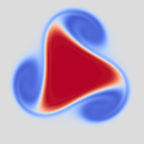
- A Mode 3 vortex instability (equidistant grid)
- Divergence test for a vortex instability on an adaptive grid
- Tracers in an accelerating frame of reference
- Tracers and buoyancy
- Internal waces and the dispersion relation
- 2D Rayleigh-Benard convection
- A dipole-Wall collision on an adaptive grid
- Vortex-ring collision (3D adaptive test)
Examples
To do
- ~
Proper box boundaries (stratified flows)~ - ~
Three dimensional simulations~ - ~
Critical evaluation~