sandbox/alimare/README

My Sandbox

Welcome to my sandbox. I sort out the pages under /sandbox/alimare. My main topics of research is the development of numerical for multiphase flows.

To that end, I developed a hybrid level-set/embedded boundary numerical method (LSEB) and a thinning algorithm for the VOF function.

The LSEB method

Preliminary remark

Please note that this method is still under testing and the associated webpages may not be up to date. Feel free to contact me via the user’s forum if some of the descriptions are nebulous.

General description

The level-set is a method initially designed to study the motion by a velocity field \boldsymbol{v} of an interface \Gamma of codimension 1 that bounds several open regions \Omega (possibly connected). The main idea is to use a function \phi sufficiently smooth (Lipschitz continuous for instance) and define the interface as the 0-level-set of \phi: \displaystyle \forall \boldsymbol{x}\in\Gamma\hspace{0.1cm} , \hspace{0.2cm} \phi(\boldsymbol{x},t) = 0 My solver for using a level-set function is given in the level set page. It is meant to be used in combination with the embedded boundary method. That defines cell fractions cs and face fractions fs. In this paradigm two sets of passive scalars, tracers and tracers2 (e.g. the temperature of the liquid and the solid) can be defined, one set will be advected and/or diffused inside the 0-level-set, i.e for cells where: \displaystyle \forall \boldsymbol{x}\in\Gamma\hspace{0.1cm} , \hspace{0.2cm} \phi(\boldsymbol{x},t) \leq 0 and the other set where \phi(\boldsymbol{x},t) \geq 0.

When combined with AMR, restriction, prolongation must be redefined for the complementary metrics: \displaystyle cs_2 = 1-cs\\ fs_2.x = 1-fs.x this is done in double_embed-tree.h. To switch from a metric to the complementary one, I defined the invertcs function.

The interface is advected and follows with the classical equation: \displaystyle \partial_t\phi+\mathbf{v_{pc}}\cdot\nabla \phi=0 where \mathbf{v_{pc}} is the phase change velocity field. In my case this velocity field is defined in phase_change_velocity. In this routine, the velocity is only calculated in interfacial cells and follows the Stefan law. The velocity field is then reconstructed in the vicinity of the interface using LS_recons(). The combination of these two functions is done in LS_speed() and modifies a vector field to a phase change velocity field that can be used for advection.

I have coded several simple explicit cell-centered finite difference advection solvers (Forward Euler, Runge-Kutta 2, Runge-Kutta 3) that can be found [here] (simple_discretization.h) and have been tested here. These solvers use a cell-centered velocity field, v_{pc} being a cell-centered quantity. The timestep for these solvers must ignore the metric. Therefore, I have also defined my own timestep function timestep_LS().

Notes : The level-set does not see the metric due to the embedded boundary, but could be subject to a real metric, e.g. for axisymmetric simulations, Jose-Maria has been working on having a double metric (embedded boundary + axisymmetric), I have not tried to integrate his related patch.

When the velocity has a non-zero tangential component in the level-set advection equation, there is a local diffusion and smearing of the interface. The zero level-set should be correct but we get wrong isovalues after a certain time due to the crossing of characteristics of the flow. Because we use the values of the level-set function in the vicinity of the 0-level-set to reconstruct a velocity field, we need to correct the values of the level-set to get |\nabla \phi | = 1 or at least ensure a Lipschitz continuity. A common way of correcting the distance function, is to iterate on the following Hamilton-Jacobi equation: \displaystyle \left\{\begin{array}{ll} \phi_\tau + sign(\phi^{0}) \left(\left| \nabla \phi\right| - 1 \right) = 0\\ \phi(x,0) = \phi^0(x) \end{array} \right. where \tau is a fictitious time and \phi^0 is the value of \phi at the beginning of the redistancing process. This is done in the LS_reinit() function. Validation test cases are:

• Reinit_1D
• Reinit_LS
• Reinit_circle
• Zalesak circle
• Rider & Kothe’s snake (which is a variation of the Scardovelli & Zaleski’s test case). It tests the ability of the reinitialization function with an important smearing of an interface.

Sometimes, a new cell becomes uncovered because the interface has moved, in this cell, we must initialize the tracer fields. For that we use Ghigo’s methodology in update_tracer() that can be found in this page. The basic idea is very similar to what can be found in the Dirichlet boundary condition calculation in embed.h.

Curvature of the 0-level-set can also be calculated see here with similar results to the basilisk’s VOF curvature calculation

But how do I use this ?

For now you have to use a combination of header files, I list here some …

All of these routines are combined in a big black box advection_LS() that can be used as such (well, with a few adjustable parameters…). Another required header file is the level-set which is an embryo of all a full solver To do mesh adaptation with variables defined inside and outside of the emebedded boundary, operators have to be defined, this is done in this file CFL condition must be redefined with a continuous field that ignores the embedded boundary, this is done combining my definition of the timestep and functions defined in LS_advection.h.

Validation test cases

Validation test cases can be found on the following pages:

• 1D-solidifying planar interface. Fixed timestep
• 1D-solidifying planar interface
• 2D-melting crystal with a Gibbs-Thomson condition on the interface
• The Mullins-Sekerka instability
• 2D crystal growth with a Gibbs-Thomson condition
• Linear solvability test case
• Grid resolution effect on crystal growth

Application cases

• Rayleigh-Benard instability with a melting boundary

Skeletons

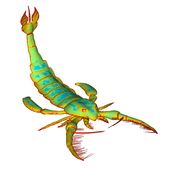
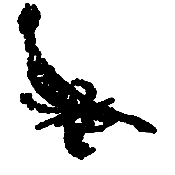
Recently I have started working on the construction of skeletons using the VOF tracer and thinning algorithms. The method works in parallell in 2D and sequentially in 3D.

• Two functions for thinning a binary field

A few examples can be found here:

• Time reversed skeleton of a level-set
• Skeleton of an STL file
• Skeleton of a 2D atomisation

Future work will focus on 3D atomisation and control of the dynamics of under-resolved structures when using a VOF tracer (ligament pinching, liquid sheet perforation…).

Miscalleneous functions

Most of the little functions that I use (e.g. biquadratic, bilinear interpolation, L_2-norm…) can be found in alex_functions.h. It also contains a few predefined Constructive Solid Geometry forms. A good description of this technique is given in Alexis Berny’s sandbox.

See also