src/test/geo.c
Geostrophic adjustment
This test case was originally proposed by Leroux et al., 1998 and Dupont, 2001 and is also discussed in Popinet & Rickard, 2007, section 6.1.
We consider the geostrophic adjustment problem studied by Dupont and Le Roux et al.. A Gaussian bump \displaystyle \eta ( x, y ) = \eta_0 e^{^{- \frac{x^2 + y^2}{R^2}}} is initialised in a 1000 \times 1000 km, 1000 m deep square basin. A reduced gravity g = 0.01 m/s^2 is used to approximate a 10 m-thick stratified surface layer. On an f-plane the corresponding geostrophic velocities are given by \displaystyle \begin{aligned} u ( x, y ) & = \frac{2 g \eta_0 y}{f_0 R^2} e^{- \frac{x^2 + y^2}{R^2}},\\ v ( x, y ) & = - \frac{2 g \eta_0 x}{f_0 R^2} e^{- \frac{x^2 + y^2}{R^2}}, \end{aligned} where f_0 is the Coriolis parameter. Following Dupont we set f_0 = 1.0285 \times 10^{- 4} s^{- 1}, R = 100 km, \eta_0 = 599.5 m which gives a maximum geostrophic velocity of 0.5 m/s.
In the context of the linearised shallow-water equations, the geostrophic balance is an exact solution which should be preserved by the numerical method. In practice, this would require an exact numerical balance between terms computed very differently: the pressure gradient and the Coriolis terms in the momentum equation. If this numerical balance is not exact, the numerical solution will adjust toward numerical equilibrium through the emission of gravity-wave noise which should not affect the stability of the solution. This problem is thus a good test of both the overall accuracy of the numerical scheme and its stability properties when dealing with inertia–gravity waves. We note in particular that a standard A-grid discretisation would develop a strong computational-mode instability in this case. Also, as studied by Leroux et al, an inappropriate choice of finite-element basis functions will result in growing gravity-wave noise.
set xlabel 'Time (days)'
set ylabel 'Maximum error on surface height (m)'
plot 'log' index 'Beta = 0' u 1:2 w l t ''
Evolution of the maximum error on the surface height for the geostrophic adjustment problem. (script)
|
|
|
|
|
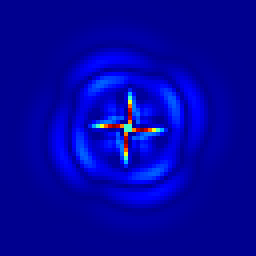
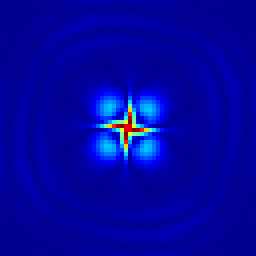
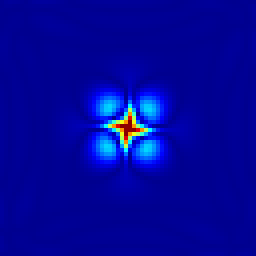
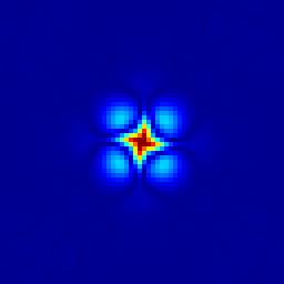
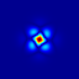
Evolution of the surface-height error field. From left to right: t = 1.157, 2.315, 3.472, 4.630, 17.361 days.
A variant of this test case uses a \beta-plane approximation for the Coriolis parameter: f = f_0 + \beta y with \beta = 1.607\times 10^{-11} m-1s-1. The numerical energy dissipation is displayed below. Note that this looks larger than for the Gerris equivalent case (as published in Popinet & Rickard, 2007) because the proper reference for (available) potential energy is used here, which was not the case for the Gerris case.
set ylabel 'Normalised energy'
set key center right
plot 'log' index 'Beta = 1.607e-11' u 1:($3 + $4) w l t 'Total',	\
     'log' index 'Beta = 1.607e-11' u 1:4 w l t 'Potential',            \
     'log' index 'Beta = 1.607e-11' u 1:3 w l t 'Kinetic'
Evolution of the total energy for the \beta-plane geostrophic adjustment problem. (script)
References
| [popinet2007] |
S. Popinet and G. Rickard. A tree-based solver for adaptive ocean modelling. Ocean Modelling, (16):224–249, 2007. [ .pdf ] |
| [dupont2001] |
F. Dupont. Comparison of numerical methods for modelling ocean circulation in basins with irregular coasts. PhD thesis, McGill University, Montreal, 2001. [ .pdf ] |
| [leroux1998] |
Daniel Y Le Roux, Andrew Staniforth, and Charles A Lin. Finite elements for shallow-water equation ocean models. Monthly Weather Review, 126(7):1931–1951, 1998. |
See also
#include "grid/multigrid.h"

#include "layered/hydro.h"
#include "layered/implicit.h"

double F0 = 0., Beta = 0.;
#define F0() (F0 + Beta*y)
#include "layered/coriolis.h"

#define H0 1000.
#define R0 100e3
#define ETA0 599.5

int main()
{
  size (1000e3);
  origin (-L0/2., -L0/2.);
  init_grid (64);
  G = 0.01;
  F0 = 1.0285e-4;
  //  TOLERANCE = 1e-6;
  linearised = true;
  DT = 1000;
  //  theta_H = 0.55;
  fprintf (stderr, "# Beta = %g\n", Beta);
  run();

  Beta = 1.607e-11;
  fprintf (stderr, "\n\n# Beta = %g\n", Beta);
  run();
}

scalar h1[];

event init (i = 0)
{
  foreach() {
    zb[] = - H0; // this is important to define the reference level
		 // for (available) potential energy
    h[] = h1[] = H0 + ETA0*exp (-(x*x + y*y)/(sq(R0)));
    u.x[] = 2.*G*ETA0*y/(F0*sq(R0))*exp (-(x*x + y*y)/(sq(R0)));
    u.y[] = - 2.*G*ETA0*x/(F0*sq(R0))*exp (-(x*x + y*y)/(sq(R0)));
  }
}

scalar e[];

double error()
{
  double max = 0.;
  foreach(reduction(max:max)) {
    e[] = fabs (h1[]  - h[]);
    if (e[] > max) max = e[];
  }
  return max;
}

typedef struct {
  double ke, pe;
} Energy;

Energy energy()
{
  double KE = 0., PE = 0.;
  foreach(reduction(+:KE) reduction(+:PE)) {
    KE += h[]*(sq(u.x[]) + sq(u.y[]))/2.*dv();
    PE += G*sq(eta[])/2.*dv();
  }
  return (Energy){KE, PE};
}

event movie (i += 10) {
  output_ppm (e, file = "e.mp4", n = 256, spread = -1);
}

event logfile (i += 1; t <= 20.*86400) {
  static Energy E0 = {0.,0.};
  Energy E = energy();
  if (i == 0)
    E0 = E;
  double Etot0 = E0.ke + E0.pe;
  fprintf (stderr, "%g %g %.8g %.8g %g\n", t/86400., error(),
	   E.ke/Etot0, E.pe/Etot0, dt);
}

event plots (i = 100; i += 100)
{
  if (Beta == 0.) {
    char s[80];
    sprintf (s, "e-%g.png", t/86400.);
    output_ppm (e, file = s, spread = -1, n = 256);
  }
}