sandbox/huet/tests/lagrangian_caps/rbc_shear.c

Red Blood Cell (RBC) in a shear flow

Definition of the relevant parameters

We define the following physical quantities:

• the size of the box L_0 = 4,
• the radius a = 1,
• the shear rate \dot{\gamma} = 1,
• the Reynolds number Re \ll 1,
• the viscosity \mu = 1,
• the density \rho = \frac{Re \, \mu}{\dot{\gamma} a^2},
• the Capillary number defined - in the case of capsules - as the ratio of viscous forces over elastic forces: Ca = \frac{\mu a \dot{\gamma}}{E_S}
• the elastic modulus E_s
• the area dilatation modulus C
• the bending modulus E_b, but it is more convenient to consider the non-dimensional bending modulus \tilde{E}_b = \frac{E_b}{a^2 E_s}
• the (global) reference curvature is switched on: c_0 = -2.09/a

#define L0 4.
#define RADIUS 1.
#define SHEAR_RATE 1.
#ifndef RE
  #define RE 0.01
#endif
#define MUP 1.
#define MUC 5.
#define RHO (RE*MUP/(SHEAR_RATE*sq(RADIUS)))
#ifndef CA
  #define CA 0.1
#endif
#define E_S (MUP*RADIUS*SHEAR_RATE/CA)
#define ND_EB .01
#define E_B (ND_EB*E_S*sq(RADIUS))
#define REF_CURV 1
#define GLOBAL_REF_CURV 1
#define C0 (-2.09/RADIUS)
#define AREA_DILATATION_MODULUS 50.

We also define some solver-ralated quantities:

• the non-dimensional duration time of the simulation TEND
• the minimum and maximum refinement levels of the Eulerian grid
• the number of Lagrangian points NLP on the capsule
• the maximum time-step DT_MAX, which appears to be limited by the bending stresses
• the tolerance of the Poisson solver (maximum admissible residual)
• the tolerance of the wavelet adaptivity algorithm for the velocity
• the stokes boolean, in order to ignore the convective term in the Navier-Stokes solver
• the Jacobi preconditionner, which we turn on for this case.
• the output frequency: a picture is generated every OUTPUT_FREQ iterations

#ifndef TEND
  #define TEND (30./SHEAR_RATE)
#endif
#ifndef MINLEVEL
  #define MINLEVEL 4
#endif
#ifndef MAXLEVEL
  #define MAXLEVEL 6
#endif
#ifndef LAG_LEVEL
  #define LAG_LEVEL 4
#endif
#ifndef DT_MAX
  #define DT_MAX 1.e-4
#endif
#ifndef MY_TOLERANCE
  #define MY_TOLERANCE 1.e-3
#endif
#ifndef U_TOL
  #define U_TOL 0.01
#endif
#ifndef OUTPUT_FREQ
  #define OUTPUT_FREQ 100
#endif
#ifndef STOKES
  #define STOKES true
#endif
#define JACOBI 1

Simulation setup

We import the octree grid, the centered Navier-Stokes solver, the Lagrangian mesh, the Skalak elastic law, the bending force in the front-tracking context, the viscosity ratio for capsules, a header file containing functions to mesh a sphere, and the Basilisk viewing functions supplemented by a custom function draw\_lag useful to visualize the front-tracking interface.

#include "grid/octree.h"
#include "navier-stokes/centered.h"
#include "lagrangian_caps/capsule-ft.h"
#include "lagrangian_caps/skalak-ft.h"
#include "lagrangian_caps/bending-ft.h"
#include "lagrangian_caps/viscosity-ft.h"
#include "lagrangian_caps/common-shapes-ft.h"
#include "lagrangian_caps/view-ft.h"

FILE* foutput = NULL;

const scalar myrho[] = RHO;
const face vector myalpha[] = {1./RHO, 1./RHO, 1./RHO};

int main(int argc, char* argv[]) {
  origin(-0.5*L0, -0.5*L0, -0.5*L0);

We set periodic boundary conditions on the non-horizontal walls.

  periodic(top);
  periodic(front);
  N = 1 << MAXLEVEL;
  rho = myrho;
  alpha = myalpha;
  TOLERANCE = MY_TOLERANCE;

We don’t need to compute the convective term in this case, so we set the boolean stokes to false. However it is still important to choose Re \ll 1 since we are solving the unsteady Stokes equation.

  stokes = STOKES;
  DT = DT_MAX;
  run();
}

We impose shear-flow boundary conditions…

u.n[left] = dirichlet(0);
u.n[right] = dirichlet(0);
u.r[left] = dirichlet(0.);
u.r[right] = dirichlet(0.);
u.t[left] = dirichlet(-SHEAR_RATE*x);
u.t[right] =  dirichlet(-SHEAR_RATE*x);
uf.n[left] = dirichlet(0);
uf.n[right] = dirichlet(0);

event init (i = 0) {

… and we initialize the flow field to that of an undisturbed, fully-developed shear.

  foreach() {
    u.x[] = 0.;
    u.y[] = -SHEAR_RATE*x;
    u.z[] = 0.;
  }

We initialize a biconcave membrane using the pre-defined function in common-shapes-ft.h

  activate_biconcave_capsule(&CAPS(0), level = LAG_LEVEL, radius = RADIUS);
  foutput = fopen("output.txt","w");
}

The Eulerian mesh is adapted at every time step, according to two criteria:

• first, the 5x5x5 stencils neighboring each Lagrangian node need to be at a constant level. For this purpose we tag them in the stencil scalar, which is fed to the adapt\_wavelet algorithm,
• second, we adapt according to the velocity field.

event adapt (i++) {
  tag_ibm_stencils(&CAPS(0));
  adapt_wavelet({stencils, u}, (double []){1.e-2, U_TOL, U_TOL, U_TOL},
    minlevel = MINLEVEL, maxlevel = MAXLEVEL);
  generate_lag_stencils(&CAPS(0));
}

We also output a movie frame every OUTPUT_FREQ iteration

event pictures (i+=OUTPUT_FREQ) {
  char name[32];
  view(fov = 18.9, bg = {1,1,1}, psi=pi/2.);
  clear();
  cells(n = {0,0,1});
  squares("u.y", n = {0,0,1}, map = cool_warm);
  draw_lag(&CAPS(0), lw = 1, edges = true, facets = true, fc = {1., 1., 1.});
  sprintf(name, "ux_%d.png", i);
  save(name);

  view(fov = 18.9, bg = {1,1,1}, theta = pi/10, psi=pi/2.);
  clear();
  // cells(n = {0,0,1});
  draw_lag(&CAPS(0), lw = 1, edges = true, facets = true, fc = {156./255, 22./255, 9./255});
  sprintf(name, "rbc_%d.png", i);
  save(name);

  view(fov = 18.9, bg = {1,1,1}, psi=pi/2.);
  clear();
  cells(n = {0,0,1});
  squares("I", n = {0,0,1}, map = cool_warm);
  sprintf(name, "viscosity_%d.png", i);
  save(name);
}

event dump (t += 1.) {
  dump(file = "dump");
  dump_capsules("dump_mbs");
}

event end (t = TEND) {
  fclose(foutput);
  return 0.;
}

Results

The command to generate the videos above from the simulation results:

ffmpeg -y -framerate 25 -i rbc_%d.png -c:v libx264 -vf "format=yuv420p" rbc.mp4

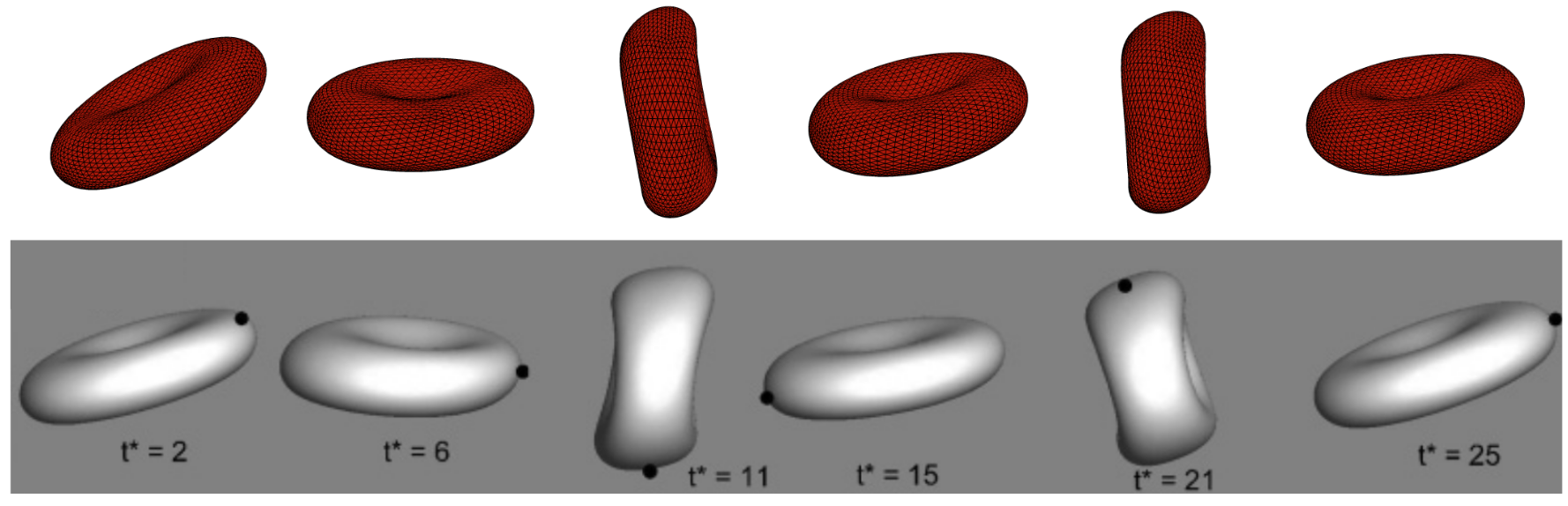
Qualitative comparison of the tumbling motion with Yazdani & Bagchi (PRE, 2011)

We observe that the RBC is undergoing a tumbling motion, a behavior of RBCs that is not seen without viscosity ratio in this range of Capillary numbers. Moreover, the deformation of the RBC matches qualitatively well that Yazdani & Bagchi. However our tumbling period seems slightly shorter than that of Yazdani & Bagchi: we attribute this small discrepancy to the fact that we may have set different values for the area dilatation modulus C, as Yazdani & Bagchi only provides a range of values: C ∈ [50, 400]. Nevertheless, the results above show that in our implementation, the combination of elastic forces, bending forces and visocity ratio matches well the qualitative results observed in the literature, and that the overall agreement is satisfactory.

References