sandbox/ghigo/src/test-navier-stokes/cylinder-strouhal.c
Flow past a fixed cylinder at different Reynolds number: Strouhal number
This test case is the analog of the Bénard–von Kármán Vortex Street for the flow around a cylinder at Re=160. A similar test case was also used in Gerris: strouhal.
We compute here the Strouhal number St=\frac{f_0 d}{u}, where f_0 is the shedding frequency of the vortex street, for different Reynolds numbers 200 \leq Re=\frac{UD}{\nu} \leq 500.
We solve here the Navier-Stokes equations and add the cylinder using an embedded boundary.
#include "grid/quadtree.h"
#include "../myembed.h"
#include "../mycentered.h"
#include "view.h"
Reference solution
#define d    (1.) // Cylinder characteristic length
#define uref (1.) // Reference velocity, uref
#define tref ((d)/(uref)) // Reference time, tref=d/u
We vary the Reynolds number between 200 and 500.
double Re = 200.; // Particle Reynolds number Re = ud/nuWe also define the shape of the domain.
#if SHAPE == 1 // Square cylinder
#define cylinder(x,y) (union (						\
			      union ((x) - (d)/2., -(x) - (d)/2.),	\
			      union ((y) - (d)/2., -(y) - (d)/2.)))
#elif SHAPE == 2 // Rectangular cylinder
#define cylinder(x,y) (union (						\
			      union ((x) - (d), -(x) - (d)),		\
			      union ((y) - (d)/2., -(y) - (d)/2.)))
#else // circular cylinder
#define cylinder(x,y) (sq ((x)) + sq ((y)) - sq ((d)/2.))
#endif // SHAPE
#define EPS (1.e-12)
coord p_p;

void p_shape (scalar c, face vector f, coord p)
{
  vertex scalar phi[];
  foreach_vertex()
    phi[] = (cylinder ((x - p.x), (y - p.y)));
  boundary ({phi});
  fractions (phi, c, f);
  fractions_cleanup (c, f,
		     smin = 1.e-14, cmin = 1.e-14);
}
Setup
We need a field for viscosity so that the embedded boundary metric can be taken into account.
face vector muv[];We define the mesh adaptation parameters.
#define lmin (6) // Min mesh refinement level (l=6 is 2pt/d)
#define lmax (11) // Max mesh refinement level (l=11 is 64pt/d)
#define cmax (1.e-3*(uref)) // Absolute refinement criteria for the velocity field

int main ()
{
The domain is 32\times 32.
We set the maximum timestep.
DT = 1.e-2*(tref);We set the tolerance of the Poisson solver.
  TOLERANCE    = 1.e-6;
  TOLERANCE_MU = 1.e-6*(uref);

  for (Re = 200.; Re <= 500.; Re += 300.) {
We initialize the grid.
Boundary conditions
We use inlet boundary conditions.
u.n[left] = dirichlet ((uref));
u.t[left] = dirichlet (0);
p[left]   = neumann (0);
pf[left]  = neumann (0);

u.n[right] = neumann (0);
u.t[right] = neumann (0);
p[right]   = dirichlet (0);
pf[right]  = dirichlet (0);
We give boundary conditions for the face velocity to “potentially” improve the convergence of the multigrid Poisson solver.
uf.n[left]   = (uref);
uf.n[bottom] = 0;
uf.n[top]    = 0;
Properties
event properties (i++)
{
  foreach_face()
    muv.x[] = (uref)*(d)/(Re)*fm.x[];
  boundary ((scalar *) {muv});
}
Initial conditions
We set the viscosity field in the event properties.
mu = muv;We use “third-order” face flux interpolation.
#if ORDER2
for (scalar s in {u, p, pf})
s.third = false;
#else
for (scalar s in {u, p, pf})
s.third = true;
#endif // ORDER2We use a slope-limiter to reduce the errors made in small-cells.
#if SLOPELIMITER
for (scalar s in {u}) {
s.gradient = minmod2;
}
#endif // SLOPELIMITER
#if TREEWhen using TREE and in the presence of embedded boundaries, we should also define the gradient of u at the cell center of cut-cells.
#endif // TREEWe initialize the embedded boundary.
We first define the cylinder’s position.
p_p.x = -(L0)/4. + (EPS);
p_p.y = (EPS);
#if TREEWhen using TREE, we refine the mesh around the embedded boundary.
astats ss;
int ic = 0;
do {
ic++;
p_shape (cs, fs, p_p);
ss = adapt_wavelet ({cs}, (double[]) {1.e-30},
maxlevel = (lmax), minlevel = (1));
} while ((ss.nf || ss.nc) && ic < 100);
#endif // TREE
p_shape (cs, fs, p_p);We also define the volume fraction at the previous timestep csm1=cs.
csm1 = cs;We define the no-slip boundary conditions for the velocity.
u.n[embed] = dirichlet (0);
u.t[embed] = dirichlet (0);
p[embed] = neumann (0);
uf.n[embed] = dirichlet (0);
uf.t[embed] = dirichlet (0);
pf[embed] = neumann (0);We initialize the velocity.
Embedded boundaries
Adaptive mesh refinement
#if TREE
event adapt (i++)
{
adapt_wavelet ({cs,u}, (double[]) {1.e-2,(cmax),(cmax)},
maxlevel = (lmax), minlevel = (1));We also reset the embedded fractions to avoid interpolation errors on the geometry. This would affect in particular the computation of the pressure contribution to the hydrodynamic forces.
p_shape (cs, fs, p_p);
}
#endif // TREEOutputs
double CD = 0., CL = 0.;
event init (i = 0)
{
CD = 0., CL = 0;
}
event coeffs (i++; t <= 100.*(tref))
{
coord Fp, Fmu;
embed_force (p, u, mu, &Fp, &Fmu);
CD = (Fp.x + Fmu.x)/(0.5*sq ((uref))*(d));
CL = (Fp.y + Fmu.y)/(0.5*sq ((uref))*(d));
char name1[80];
sprintf (name1, "Re-%.0f.dat", Re);
static FILE * fp = fopen (name1, "w");
fprintf (fp, "%g %d %g %g %d %d %d %d %d %d %g %g %g %g %g %g\n",
(Re),
i, t/(tref), dt/(tref),
mgp.i, mgp.nrelax, mgp.minlevel,
mgu.i, mgu.nrelax, mgu.minlevel,
mgp.resb, mgp.resa,
mgu.resb, mgu.resa,
CD, CL);
fflush (fp);
}
event logfile (t = end)
{
fprintf (stderr, "%g %g %g %d %d %d %d %d %d %g %g %g %g %g %g\n",
(Re),
t/(tref), dt/(tref),
mgp.i, mgp.nrelax, mgp.minlevel,
mgu.i, mgu.nrelax, mgu.minlevel,
mgp.resb, mgp.resa,
mgu.resb, mgu.resa,
CD, CL);
fflush (stderr);
}Snapshots
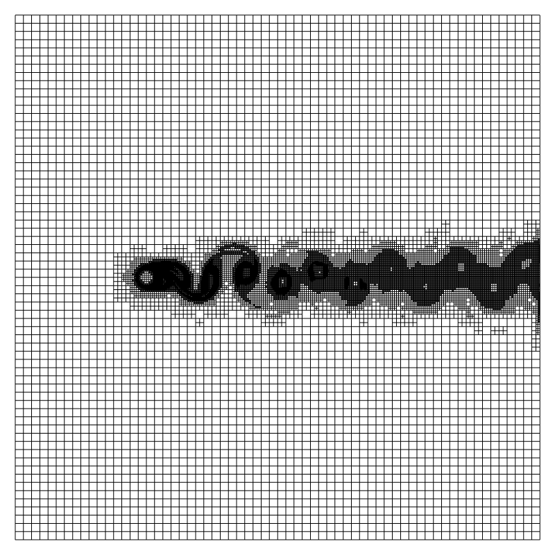
We first plot the entire domain.
clear ();
view (fov = 20, camera = "front",
tx = 0., ty = 0.,
bg = {1,1,1},
width = 800, height = 800);
draw_vof ("cs", "fs", lw = 5);
cells ();
sprintf (name2, "mesh-Re-%.0f.png", Re);
save (name2);
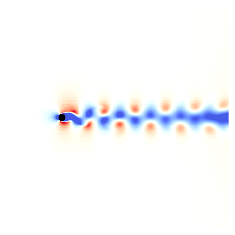
draw_vof ("cs", "fs", filled = -1, lw = 5);
squares ("u.x", map = cool_warm);
sprintf (name2, "ux-Re-%.0f.png", Re);
save (name2);
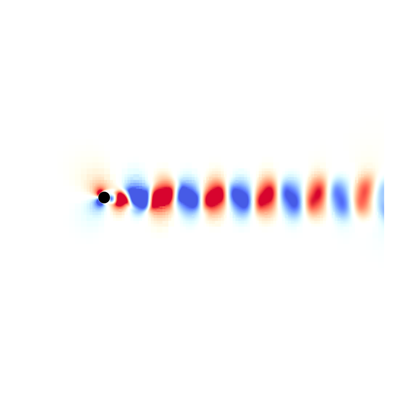
draw_vof ("cs", "fs", filled = -1, lw = 5);
squares ("u.y", map = cool_warm);
sprintf (name2, "uy-Re-%.0f.png", Re);
save (name2);
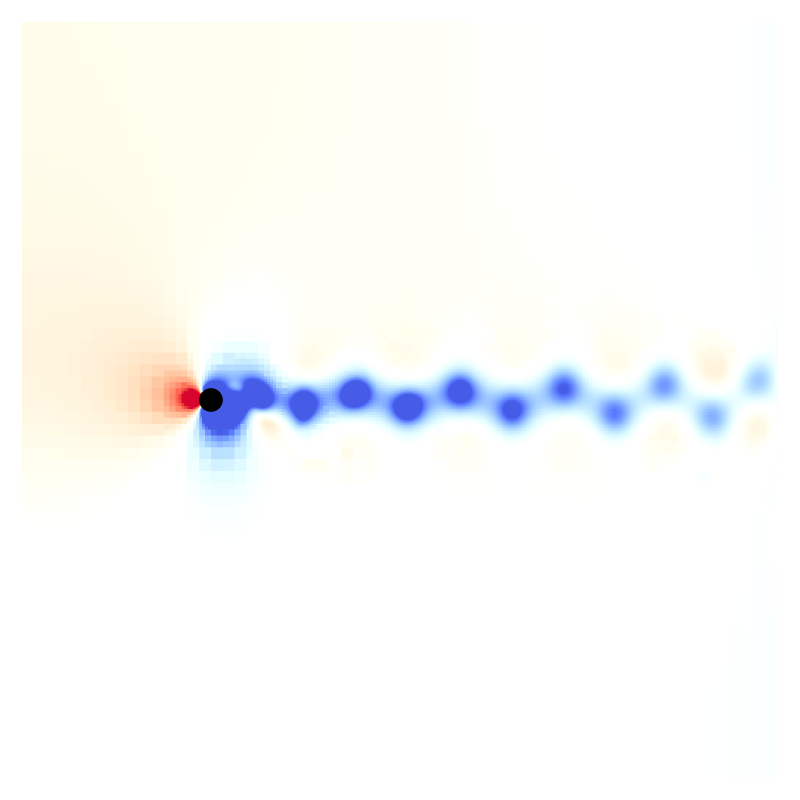
draw_vof ("cs", "fs", filled = -1, lw = 5);
squares ("p", map = cool_warm);
sprintf (name2, "p-Re-%.0f.png", Re);
save (name2);
draw_vof ("cs", "fs", filled = -1, lw = 5);
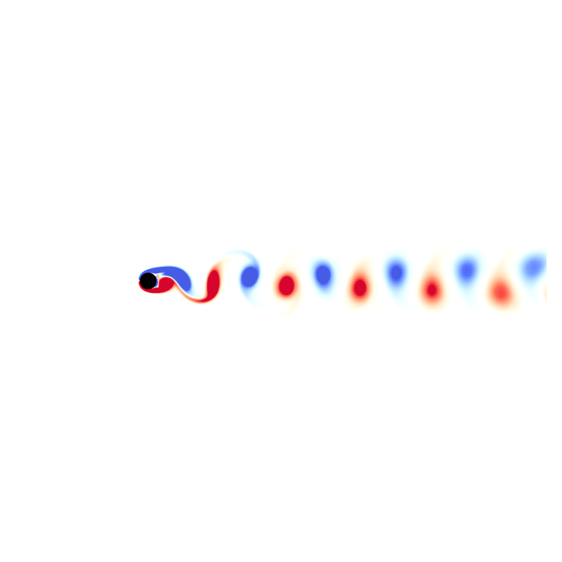
squares ("omega", map = cool_warm);
sprintf (name2, "omega-Re-%.0f.png", Re);
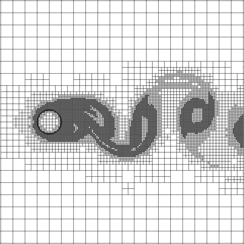
save (name2);We then zoom on the cylinder.
clear ();
view (fov = 6, camera = "front",
tx = -(p_p.x + 3.)/(L0), ty = 0.,
bg = {1,1,1},
width = 800, height = 800);
draw_vof ("cs", "fs", lw = 5);
cells ();
sprintf (name2, "mesh-zoom-Re-%.0f.png", Re);
save (name2);
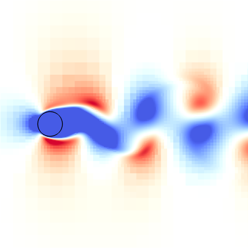
draw_vof ("cs", "fs", lw = 5);
squares ("u.x", map = cool_warm);
sprintf (name2, "ux-zoom-Re-%.0f.png", Re);
save (name2);
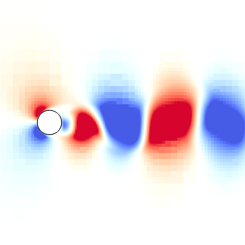
draw_vof ("cs", "fs", lw = 5);
squares ("u.y", map = cool_warm);
sprintf (name2, "uy-zoom-Re-%.0f.png", Re);
save (name2);
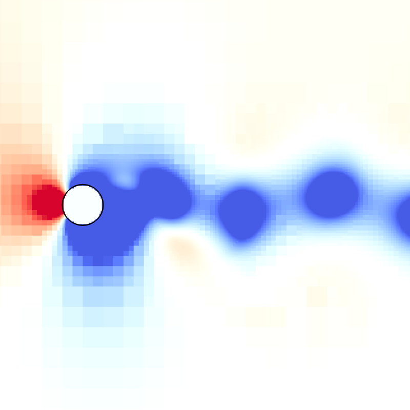
draw_vof ("cs", "fs", lw = 5);
squares ("p", map = cool_warm);
sprintf (name2, "p-zoom-Re-%.0f.png", Re);
save (name2);
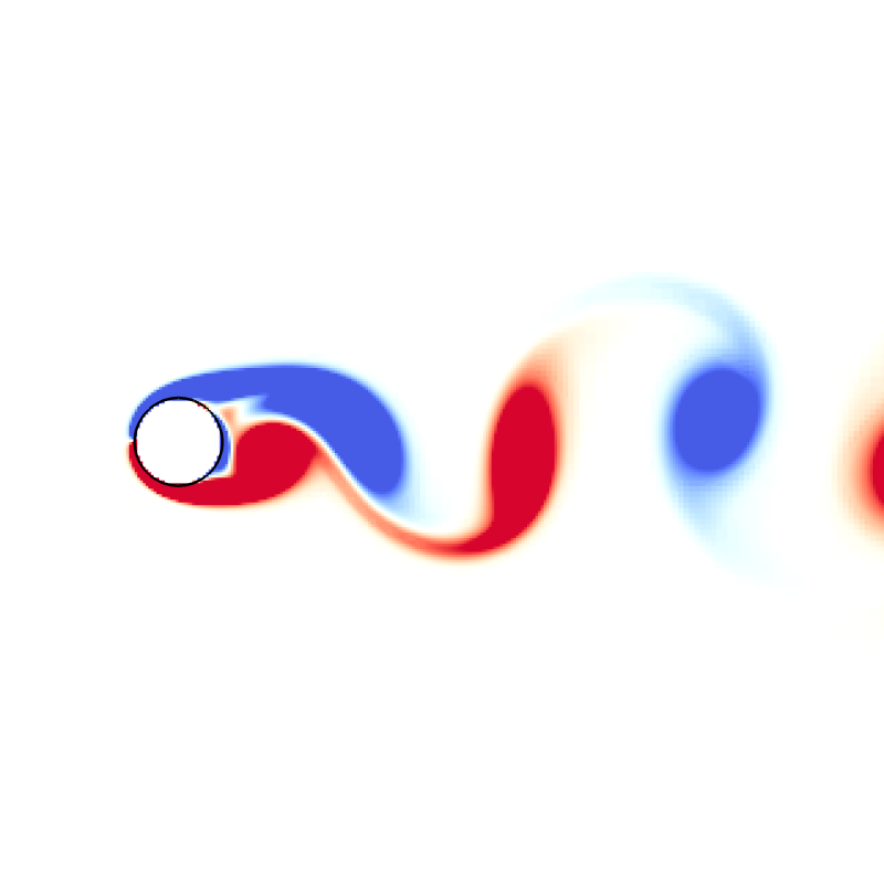
draw_vof ("cs", "fs", lw = 5);
squares ("omega", map = cool_warm);
sprintf (name2, "omega-zoom-Re-%.0f.png", Re);
save (name2);
}Results
Snapshots for Re = 200
Drag and lift coefficients
We plot the time evolution of the drag and lift coefficients C_D and C_L for different Reynolds numbers Re.
set terminal svg font ",16"
set key top right spacing 1.1
set grid ytics
set xtics 0,20,100
set xlabel 't/(d/u)'
set ylabel 'C_{D}'
set xrange[0:100]
set yrange [0:4]
plot for [i=200:500:300] \
     sprintf('Re-%i.dat',i) u 3:15 w l t sprintf('Re=%i, C_D', i)
set ylabel 'C_{L}'
set yrange [-4:4]
plot for [i=200:500:300] \
     sprintf('Re-%i.dat',i) u 3:16 w l t sprintf('Re=%i, C_L', i)
Strouhal number
We plot the Strouhal number St as a function of the Reynolds number Re. We compare the results to Williamson’s universal law Williamson, 1988 and to the results obtained with the software Gerris.
set key font ",8" top right spacing 0.6
set multiplot layout 2,1

ftitle(Re,f) = sprintf("Re=%.0f, f0=%.3f", Re, f/(2.*pi));

# Fit the lift coefficient
set fit errorvariables

f1(x) = a1*sin((x)*f1) + b1*cos((x)*f1);
a1 = 1; b1 = 1; f1=0.2*2.*pi;
fit [80:*][*:*] f1(x) 'Re-200.dat' using 3:16 via a1, b1, f1

f2(x) = a2*sin((x)*f2) + b2*cos((x)*f2);
a2 = 1; b2 = 1; f2=0.2*2.*pi;
fit [80:*][*:*] f2(x) 'Re-500.dat' using 3:16 via a2, b2, f2

set print "fit_static.dat"print 200,f1/(2.*pi),f1_err
print 500,f2/(2.*pi),f2_err
set print
# Time evolution of the lift coefficient
unset grid
set xtics 0,10,100
set ytics -10,2,10
set ylabel 'C_{L}'
set yrange[-4:4]
plot 'Re-200.dat' u ($3):($16) w l lw 3 lc rgb "black" notitle, \
f1(x) w l lw 2 lc rgb "brown" t ftitle(200, f1), \
'Re-500.dat' u ($3):($16) w l lw 3 lc rgb "dark-blue" notitle, \
f2(x) w l lw 2 lc rgb "blue" t ftitle(500, f2)
# Plot the Strouhal number
set xtics 0,50,10000
set ytics 0,0.1,1
set xlabel 'Re'
set ylabel 'St'
set xrange[150:550]
set yrange[0.1:0.5]
# Williamson law for St = f(Re)
f(x) = -3.3265/x + 0.1816 + 1.6e-4*x
plot f(x) w l lw 3 lc rgb "black" t "Williamson, 1988", \
'../data/strouhal_cylinder/gerris/static.ref' u 1:2 w lp lw 2 lc rgb "blue" t "Gerris fixed, high resolution", \
'../data/strouhal_cylinder/gerris/moving.ref' u 1:2 w lp lw 2 lc rgb "red" t "Gerris moving, high resolution", \
'fit_static.dat' u 1:2 w p pt 7 ps 1 lc rgb "sea-green" t "Basilisk"
unset multiplot
References
| [williamson1988] |
C.H.K. Williamson. Defining a universal and continuous strouhal–reynolds number relationship for the laminar vortex shedding of a circular cylinder. The Physics of Fluid, 31:2742–2744, 1988. |