sandbox/M1EMN/Exemples/airywave.c
Linearized Airy Wave Theory
Problem
How propagates the swell in open sea? It is a small perturbation of the free surface of the sea.
Equations
Here we do not use Navier Stokes like in houle.c, but instead we solve the Laplacian.
The linear perturbation of interface \eta = \eta_0 \sin(kx-\omega t) admits a potential \phi = ( \omega \cosh(k y)/sinh(H k) \eta_0 \sin(kx-\omega t) )/k with the famous dispersion relation: \omega^2=g k \tanh(k H ) so that u= \frac{k g}{\omega} \cos(kx-\omega t) \cosh(ky)/\cosh(kH ), \;\; v= \omega \sin(kx-\omega t) \sinh(ky)/ \cosh(kH ), \;\; P = \rho g\eta_0 sin(kx-\omega t) \cosh(ky)/cosh(kH ) at the surface: v= \partial \eta / \partial t= (\partial P/ \partial t) /( \rho g)
We propose to solve in two at the linearized surface: \frac{\partial \phi}{\partial t}= - g \eta \frac{\partial \eta}{\partial t}= \frac{\partial \phi}{\partial y} and \frac{\partial^2 \phi }{\partial x^2}+ \frac{\partial^2 \phi }{\partial y^2}=0 and find transverse velocity \frac{\partial \phi}{\partial y}=0 at the bottom
 set arrow from 4,0 to 4,1 front
 set arrow from 4,1 to 4,0 front
 set arrow from 0.1,.1 to 9.9,0.1 front
 set arrow from 9.1,.1 to 0.1,0.1 front
 set label  "L0" at 6,.15 front
 set label  "depth H" at 4.2,.5 front
 set label  "water" at 1.2,.9 front
 set label  "air" at 1.2,1.05 front
 set xlabel "x"
 set ylabel "h"
 p [0:10]0 not,1+0.075*(cos(2*pi*x/5)+0.22121*cos(4*pi*x/5)) w filledcurves x1 linec 3 t'free surface'
Code
#include "run.h"
#include "poisson.h"

#define MAXLEVEL 7
#define G 1
double tmax;
double dt;
double H;
#define k 4*(2*pi/L0)
#define A 1//0.02*H
#define w sqrt(G*k*tanh(k*H))
#define T 2*pi/w


scalar phi[], phiS[],eta[];
scalar s0[],dphidy[];
mgstats mgp;
trick define a \phi and a \phi_S valid in the volume. Only the value of \phi_S at the surface as a physical meaning. The bulk value has no meaning
phi[top] = dirichlet(phiS[]);
phi[bottom] = neumann(0);
phiS[bottom] = neumann(0);
eta[bottom] = neumann(0);

event init (i = 0)
{
  mask (y >  H ? top :    none);

  foreach()
    phiS[] =  (G/w*sin(k*x)) ;
  boundary ({phiS});

  foreach()
    eta[] = A*cos(k*x) ; // exp(-(x-2.5)*(x-2.5)/.1);//sin(2*pi*x/L0);
  boundary ({eta});

  foreach()
    phi[] = (A*w/k)*(cosh(k*y)/sinh(H*k))*sin(k*x) ;
  boundary ({phi});
source 0 of Laplacian
int main()
{
    L0 = 10.;
    H = L0/4;
    origin(0,0);
    init_grid (1 << MAXLEVEL);
    DT = 1.e-2;
    tmax = 1 * 2*pi/w;
    periodic(right);
    run();
}
event logfile (i++)
{
//    stats s = statsf (phi);
//    fprintf (stderr, "%d %g %d %g %g %g\n",
//             i, t, mgp.i, s.sum, s.min, s.max);
}
event sauve (t +=.1;t <= tmax)
{
FILE *  fpc = fopen("Fwave.txt", "w");
 foreach()
      fprintf (fpc, "%g %g %g \n", x, y, phi[]);
 fclose(fpc);

      fprintf (stderr, " ~~~~~~~~~~~t=%lf eta(3,H)=%lf T=%lf \n",t,interpolate(eta,3.,H*0.9999999),2*pi/w);
}

#ifdef gnuX
event output (t += .1; t < tmax) {
  fprintf (stdout, "p[0:%lf][-1:2]  '-' u 1:2  not  w  p,''u 1:3 w p \n",L0);
  //was  foreach(x)
    foreach()
    fprintf (stdout, "%g %g %g \n", x,  interpolate(eta,x,H*.999), cos(k*x - w *t ));
  fprintf (stdout, "e\n\n");}

#else
event output (t += .01; t < tmax) {

  //was  foreach(x)
    foreach()
     fprintf (stdout, "%g %g %g \n", x,  interpolate(eta,x,H*0.999), t);

     fprintf (stdout, "\n");
}
#endif
Time integration
event integration (i++) {We first set the timestep according to the timing of upcoming events.
dt = dtnext (DT);Update the value of \phi^{n+1} at the surface which is the dirichlet boundary condition for the laplacian \phi^{n+1}|_S = \phi^{n}|_S - g \eta^{n}
Solve \frac{\partial^2 \phi^{n+1}}{\partial x^2}+ \frac{\partial^2 \phi^{n+1}}{\partial y^2}=0 and find transverse velocity \frac{\partial \phi^{n+1}}{\partial y}
at the surface (but every where) \eta^{n+1} = \eta^{n} +\frac{\partial \phi^{n+1}}{\partial y}|_S
    foreach()
      eta[] += dphidy[]*dt;
    boundary({eta});
}
event pictures (t=1) {
    scalar l[];
    foreach()
    l[] = phi[];
    boundary ({l});
     output_ppm (l, file = "houle.png", min = -1,   max= 1, n=512 ,  box = {{0,0},{10,10./4}} );
}
event movie (t += .25) {
   scalar l[];
    foreach()
    l[] = phi[] ;
    boundary ({l});
 //   static FILE * fp2 = popen ("ppm2mpeg > houle.mpg", "w");
 //    output_ppm (l, fp2 , min = -1,  max= 1,
 //     linear = true, n = 512 , box = {{0,0},{L0,H}});
    output_ppm (l, file = "houle.mp4"  , min = -1,  max= 1,
      linear = true, n = 512 , box = {{0,0},{L0,H}});
}
Run
Then compile and run:
qcc -O2 -Wall -DgnuX=1 -o airywave airywave.c -lm
./airywave | gnuplot
or with makefile
make airywave.tst;make airywave/plots;make airywave.c.htmlResults
Plot of the interface
 reset
 set output 'fhoule.png'
 set pm3d map
 set palette gray negative
 unset colorbox
 set xlabel "x"
 set ylabel "t"
 unset key
 splot 'out' u 1:3:2
plot of \phi
 reset
 sp 'Fwave.txt'
Animation of velocity
velocity (click on image for animation)](airywave/houle.png) 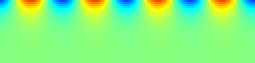
AA & PYL Paris 02/16
Links
Bibliography
- Billingham, A. C. King Wave motion
- C. & P. Aristaghes
- PYL cours sur la houle M2