sandbox/easystab/stab2014/advection-diffusion.m

March in time of the vibrating string

In this code, we simuate the evolution in time of an initial condition of a model of a guitar string, simply an elastic string tensed under two fixed attachement points. What is interesting with this system from the technical point of view is that the dynamic equation has a second derivative in time and we show here how to transform this into a larger system with just a single time derivative.

We also show hee a very simple way to do marching in time, by simply building a matrix M which if we do a matrix-vector multiplication with a given state of the string, we get the state of the string a little time later (equal to the chosen time step).

clear all; clf

% parameters
N=200; % number of gridpoints
L=70; % domain length
c=1; % wave velocity
dt=0.2; % time step
tmax=60; % final time
U=0.5;   % speed value
nu=0.2   %value of the kinematic viscosity
orig=0.5; % time in the past when the dirac started

% differentiation matrices
scale=-2/L;
[x,DM] = chebdif(N,2); 
dx=DM(:,:,1)*scale;    
dxx=DM(:,:,2)*scale^2;    
x=(x-1)/scale; 
Z=zeros(N,N); I=eye(N); 
II=eye(2*N);


% system matrices
E=I;
A=nu*dxx-dx*U;

% locations in the state
v=1:N;
f=N+1:2*N;

Boundary conditions

The original system has one variable and two time derivatives, so we should apply two boundary conditions. We will simply say that the position of the string at its both ends should be zero: two attachment points. This is a homogeneous Dirichlet condition applied on the first and last point of the state vector for the state position.

% boundary conditions
E(1,:)=0;
A(1,:)=I(1,:);
 E(N,:)=0;
 A(N,:)=I(N,:);
         


% march in time matrix 
M=(E-A*dt/2)\(E+A*dt/2);

Initial condition

We need to describe the state of the system at initial time. We say here that the string is initially deformed as a sinus (this satisfies the boundary conditions), and that the velocity is zero. From that state we then perform a loop to repeatedly advance the state of a short forward step in time. We use drawnow to show the evolution of the simulation as a movie when running the code. We store for validation the string position at the midle of the domain, to do this without worrying about the the grid points are, we interpolate f with the function interp1.

% initial condition
t0=orig;
q=(exp(-(((x-L/4).^2)/(4*nu*t0))))/(2*sqrt(pi*nu*t0));
qq=q
% marching loop
tvec=dt:dt:tmax; 
Nt=length(tvec);
e=zeros(Nt,1);

for ind=1:Nt    
    t=ind*dt;
    q=M*q; % one step forward
    e(ind)=interp1(x,q,L/2); % store center point
    
    % plotting
    qff=(exp(-(((x-U*t-L/4).^2)/(4*nu*(t+orig)))))/(2*sqrt(pi*nu*(t+orig)));
    qf=exp(-((x-t*U-L/4)/0.5).^2); 
    subplot(1,2,1);  plot(x,q,'b',x,qff,'r--',x,qq,'k'); 
   
    subplot(1,2,2);
    plot(t,norm((q-qff)/max(q),2),'b*'); grid on;hold on
    
    drawnow
end

legend('error'); title('error between the numerical solution and the analytical solution')
xlabel('t'); ylabel('error');

subplot(1,2,1);
 legend('advection_diffusion solution','analytical solution','initial condition');
    title('comparison numerical and analytical solution');
    xlabel('x'); ylabel('y');
    axis([0,L,-2,2])    

visualisation of the advected diffused solution

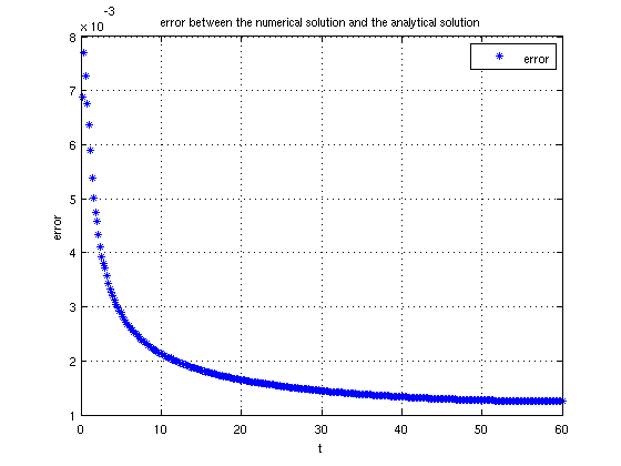
error between the numerical and the theoritical solution