sandbox/easystab/LectureNotes_Viscous.md
Viscous temporal stability analysis of parallel flows - Tollmien-Schlishting instability (chap. 7)
Introduction :
Two motivations:
What is the effect of viscosity on the inflexional instabilities (Kelvin-Helmoltz and the like) decscribed in previous paragraph ?
In boundary layers over plane plates and other profiled objects (wings,…), experiments show the existence of ustable waves called Tollmien - Schlishting waves (see also Charru, 5.1.2). However the boundary-layer velocity profiles do not display any inflection point.
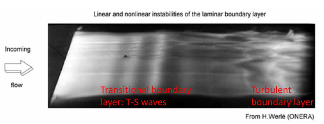
Can viscosity explain the existence of such instabilities ?
In this section we investigate the stability problem of a parallel flow including viscosity.
As in chapter 6 we restricty to 2D perturbations and to a temporal stability framework (the wavenumber k is real and the frequency \omega is complex).
Mathematical analysis
Primitive equations.
The governing equations are derived in this introductory document in the general case. For 2D perturbations of the form [u',v',p'] = \hat{q} e^{ikx-i\omega t}, the problem can be written as follows:
- i \omega {\mathcal B} \, \hat{q} = {\mathcal A} \, \hat{q}
with {\mathcal B} = \left[ \begin{array}{ccc} 1 & 0 & 0 \\ 0 & 1 & 0 \\ 0 & 0 & 0 \end{array} \right]
{\mathcal A} = \left[ \begin{array}{ccc} -i k \bar{U} + Re^{-1} ( \partial_y^2 - k^2) & - \partial_y \bar{U} & - i k \\ 0 & -i k \bar{U} + Re^{-1} ( \partial_y^2 - k^2) & - \partial_y \\ i k & \partial_y & 0 \end{array} \right]
The Orr-sommerfeld equation
Using the same manipulations as for the Rayleigh equation, one can reduce the problem to a single equation for the streamfunction component \hat \psi :
(\bar{U} - c) (\partial_y^2 - k^2) \hat \psi - \partial_y^2 \bar{U} \hat \psi = (i k Re)^{-1} (\partial_y^2 - k^2)^2 \hat \psi
Mathematical analysis of the OS equation
This equation is a fourth-ordrer differential equation which constitutes an eigenvalue problem for the eigenvalue \omega (or c).
As Re \rightarrow \infty this equation seems to approach the Rayleigh equation. However, the viscous term is a singular perturbation because it involves a small parameter multiplied by the highest-ordrer derivative (fourth-order here). Because of this property, one can expect the existence of regions where the solution displays abrupt variations in some region where the higher-order term is dominant.
In practice, the solution can display such singular phenomena in two regions :
If the flow is bounded by a wall at y= y_1 and/or y=y_2, the eigenmodes are expected to display a boundary layer behaviour. Inspection shows that the boundary layer thickness is \delta = {\mathcal O}(Re^{-1/2}).
If the phase velocity c_r matches with the velocity of the base flow at some location y_c (i.e. c_r = \bar{U}(y_c)) and the amplification rate is small (c_i \ll 1), then the corresponding eigenmode displays a critical layer singularity. Inspection shows that the characteristic thickness of this boundary layer is \delta = {\mathcal O}(Re^{-1/3}) and that the growth rate is \omega_i = {\mathcal O}(Re^{-1/3}).
In addition to these singular behaviours, another phenomena can arise if the flow is unbounded and the velocity asymptotes to a constant (for instance if \bar{U}(y) \rightarrow U_2 as y \rightarrow y_2 = + \infty). In this case one can show that the problem admits generized eigenmode solution which are not square-integrable but behave as \hat{\psi}(y) \approx e^{i \gamma y} as y \rightarrow \infty with \gamma real. Inspection shows that the corresponding frequencies belong to a continuous spectrum defined by the half-line defined by c_r = U_2; c_i \leq -k Re^{-1}.
Numerical resolution methods
- First idea : build matrix from the OS equations.
(Advantage : the problem is scalar so the matrix is dimension N. Drawbacks, the equation is fourth-order so high-order methods are mandatory; boundary conditions are difficult to impose on the streamfunction).
- Second idea : build matrix from the primitive equations.
(Minor drawback: leads to block-matrices of dimension 3N; advantages : easier to implement, can be generalized easily to 3D and/or compressible, …).
Sample results for the three main classes of flows
Class A : flows with an inflexion point (unstable in the inviscid case)
Examples : shear layers, wakes, jets.
For such flows:
- The viscosity is generally stabilizing (growth rate \omega_i is smaller than the one computed using inviscid equations).
- The instability disapears below a critical value Re_c, typically in the range Re_c \in [1-10] (Re_c \approx 1.5 for the tanh shear layer).
- Instability exists in the same range of k as predicted by inviscid theory.
- The unstable eigenmodes have a regular structure.
- The bifurcation at Re_c is supercritical in most cases.
Illustration: see program KH_temporal_viscous.m.
Class B : Flows without inflexion points which become unstable at high Re.
Examples : Plane Poiseuille flow, Blasius boundary layer, …
For such flows:
- Viscosity is first destabilizing and then
stabilizing.
- The critical Reynolds number value is in the range Re_c \in [ 500 - 5000] (520 for Blasius BL, 5772 for plane poiseuille,…)
- The range of k corresponding to instability has a non-trivial dependency with respect to Re (and tends to small k as Re becomes large).
- The unstable eigenmodes (called Tollmien-Schlishting waves) display both a boundary-layer and a critical-layer singularity (as Re \rightarrow \infty).
- The bifurcation at Re_c is subcritical in most cases.
Illustration : see programs Poiseuille_temporal_viscous.m (for computing a spectrum and plotting the eigenmodes) and TS_PlanePoiseuille.m (for parametric study and drawing of the marginal curve in the [k,Re] plane).
Class C : Flows which are linearly stable for all values of Re.
This class comprises in particular the Cylindrical Poiseuille flow and the Plane Couette flow
Paradox ! Both these flows are known to be unstable in experiments for sufficiently large Re !
The mechanism leading to transition is more complex than linear modal 2D instability…
Exercices
Exercice 1 Squire theorem
Consider 3-dimensional perturbations with modal form q'= \hat{q} e^{i k x + i \beta z - i \omega t}. Show that the stability problem reduces to an equivalent 2D problem considering the transformation:
\tilde{k} = \sqrt{k^2+\beta^2} ; \quad \tilde{\omega} \frac{k}{\sqrt{k^2+\beta^2}} \omega ; \quad \tilde{Re} = \frac{k}{\sqrt{k^2+\beta^2}} Re
Deduce that 2D instability always appears at lower Re compared to 3D instability.