initial_conditions_dimonte_fft2.h

Initializing an interface using a given spectrum
References

Initializing an interface using a given spectrum

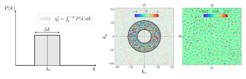
Consider \eta(x, y) being a zero mean, periodic initial perturbation at the interface between two fluids. This perturbation is further characterized by the horizontal discrete Fourier modes \hat{\eta} of wavevector \vec{k} = (k_x, k_y)^T \in \mathbb{Z}^2 and modulus k = \vert\vert k \vert\vert such that

\eta(x,y) = \sum \hat{\eta}(\vec{k}) e^{i(k_x x + k_y y)}

The realizability condition, \eta \in \mathbb{R}, imposes that for the complex Fourier modes \hat{\eta}(-\vec{k}) = \hat{\eta}^*(\vec{k}).

We further consider an annular spectrum for the interface perturbation as in Dimonte et al. (2004) of the form

\hat{\eta}(\vec{k}) = e^{i\phi(\vec{k})} \times \begin{cases} cst/k & \text{ for } \vert\vert k - k_0 \vert\vert \leq \Delta k/2 \\ 0 & \text{otherwise} \end{cases}

with

k_0 being the mean wavenumber
\Delta k the bandwidth of the perturbation
\phi the phase of the modes (here is randomly sampled)
\eta_0 the rms amplitude

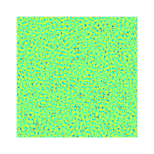
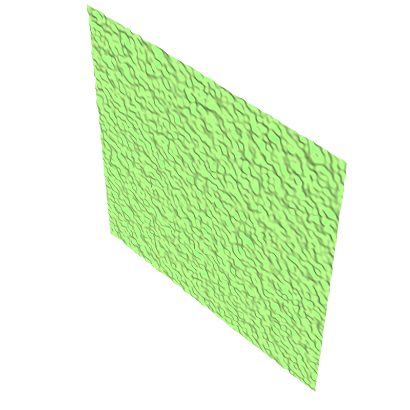
An example of the initialized interface using isvof=0 (left) and isvof=1 (right).

To initialize the interface we’ll use a Fourier transform and some interpolation routines from GSL.

#include <gsl/gsl_fft_complex.h>
#include <gsl/gsl_complex.h>
#include <gsl/gsl_complex_math.h>
#include <gsl/gsl_interp2d.h>
#include <gsl/gsl_spline2d.h>
#pragma autolink -lgsl -lgslcblas
#define REAL(z,i) ((z)[2*(i)])
#define IMAG(z,i) ((z)[2*(i)+1])

Save the initial perturbation in a gnuplot-compatible format

save_data_for_gnuplot_complex(): saves a (complex) 2D array as a .dat file

void save_data_for_gnuplot_complex(double *data, int NX, int NY, const char *filename){
  FILE *file = fopen(filename, "w");
  if (file == NULL){
    fprintf(stderr, "Error opening file %s\n", filename);
    return;
  }

  for (int i = 0; i < NX; i++){
    double kx = (i <= NX / 2) ? (2. * pi * i / L0) : (2. * pi * (i - NX) / L0);
    for (int j = 0; j < NY; j++){
      double ky = (j <= NY / 2) ? (2. * pi * j / L0) : (2. * pi * (j - NY) / L0);
      int index = i * NY + j;
      double magnitude = sqrt(sq(REAL(data, index)) + sq(IMAG(data, index)));
      fprintf(file, "%d %d %g %g %f %f %f\n", i, j, kx, ky, REAL(data,index), IMAG(data,index), magnitude);
    }
    fprintf(file, "\n"); 
  }
  fclose(file);
}

save_data_for_gnuplot_real(): saves a 2D array as a .dat file

void save_data_for_gnuplot_real(double *data, int NX, int NY, const char *filename){
  FILE *file = fopen(filename, "w");
  if (file == NULL){
    fprintf(stderr, "Error opening file %s\n", filename);
    return;
  }

  for (int i = 0; i < NX; i++){
    for (int j = 0; j < NY; j++){
      int index = i * NY + j;
      fprintf(file, "%d %d %f \n", i, j, data[index]);
    }
    fprintf(file, "\n"); 
  }
  fclose(file);
}

Generate the perturbation in Fourier space and return to physical space

init_2D_complex(): initializes the perturbation in Fourier space

void init_2D_complex(double *data, int n0, int n1, double kmin, double kmax, double eta0_target=1){
  double *kx = malloc(n0 * sizeof(double));
  double *ky = malloc(n1 * sizeof(double));
  double cst = eta0_target;

Calculate horizontal wavenumbers

  double dk_grid = 2.0 * pi / L0;  // Grid spacing in k-space
  for (int i = 0; i <= n0 / 2; ++i)
    kx[i] = dk_grid * i;

  for (int i = n0 / 2 + 1; i < n0; ++i)
    kx[i] = dk_grid * (i - n0);

  for (int i = 0; i <= n1 / 2; ++i)
    ky[i] = dk_grid * i;

  for (int i = n1 / 2 + 1; i < n1; ++i)
    ky[i] = dk_grid * (i - n1);

Initialize spectrum in the annular region with magnitude cst/k and random phase. To ensure the inverse FFT produces real values, we enforce Hermitian symmetry: F[N-i, N-j] = conj(F[i,j])

  memset(data, 0, 2 * n0 * n1 * sizeof(double));
  
  // Loop over all modes in the upper half-plane and set Hermitian symmetry
  for (int i = 0; i < n0; ++i){
    for (int j = 0; j < n1; ++j){
      double k = sqrt(sq(kx[i]) + sq(ky[j]));
      
      if ((k >= kmin) && (k <= kmax)){
        // Check if this is a mode we should generate (avoid duplicates due to symmetry)
        bool is_positive_half = (i < n0/2) || (i == n0/2 && j <= n1/2);
        bool is_dc = (i == 0 && j == 0);
        bool is_nyquist_x = (n0 % 2 == 0 && i == n0/2);
        bool is_nyquist_y = (n1 % 2 == 0 && j == n1/2);
        bool must_be_real = is_dc || (is_nyquist_x && is_nyquist_y);
        
        if (is_positive_half) {
          double magnitude = cst / sqrt(k);
          
          if (must_be_real) {
            // DC and Nyquist corners must be real
            REAL(data, i*n1+j) = magnitude * (noise() > 0.5 ? 1.0 : -1.0);
            IMAG(data, i*n1+j) = 0.0;
          } else {
            // General case: random phase
            double phase = noise() * pi;
            REAL(data, i*n1+j) = magnitude * cos(phase);
            IMAG(data, i*n1+j) = magnitude * sin(phase);
            
            // Set Hermitian conjugate if not on the boundary
            if (i != 0 || j != 0) {
              int conj_i = (i == 0) ? 0 : n0 - i;
              int conj_j = (j == 0) ? 0 : n1 - j;
              if (conj_i != i || conj_j != j) {  
                // Avoid setting the same point twice
                REAL(data, conj_i*n1+conj_j) = REAL(data, i*n1+j);
                IMAG(data, conj_i*n1+conj_j) = -IMAG(data, i*n1+j);
              }
            }
          }
        }
      }
    }
  }

  // Compute spectral RMS using Parseval's theorem
  // For GSL's unnormalized backward FFT: Var_real = (1/(n0*n1)) Σ|f[n]|² = Σ|F[k]|²
  double eta0_spectral = 0.;  
  for (int i = 0; i < n0; ++i){
    for (int j = 0; j < n1; ++j){
      int index = i * n1 + j;
      double mag_sq = sq(REAL(data, index)) + sq(IMAG(data, index));
      eta0_spectral += mag_sq;  
    }
  }

  fprintf(stdout, "Spectral RMS (Parseval): %g \n", sqrt(eta0_spectral));
  
  // Post-normalization: scale to achieve exact target RMS
  if (eta0_spectral > 0) {
    double scale = eta0_target / sqrt(eta0_spectral);
    for (int i = 0; i < n0 * n1; ++i) {
      REAL(data, i) *= scale;
      IMAG(data, i) *= scale;
    }
    eta0_spectral *= sq(scale);  // Update spectral energy after rescaling
    fprintf(stdout, "Rescaled by factor %g to achieve target RMS = %g\n", scale, eta0_target);
  }

  free(kx);
  free(ky);
}

fft2D(): uses the radix-2 routines to return to physical space

void fft2D(double *data, int n0, int n1){  
  
  // Inverse FFT along rows 
  for (int i = 0; i < n0; ++i){
    gsl_fft_complex_radix2_backward(data + 2 * i * n1, 1, n1);
  }

  // Inverse FFT along columns
  double *column = malloc(2 * n0 * sizeof(double));
  for (int j = 0; j < n1; ++j){
    for (int i = 0; i < n0; ++i){
      REAL(column,i) = REAL(data, i*n1 + j);
      IMAG(column,i) = IMAG(data, i*n1 + j);
    }
    gsl_fft_complex_radix2_backward(column, 1, n0);
    for (int i = 0; i < n0; ++i)
    {
      REAL(data, i*n1 + j) = REAL(column,i);
      IMAG(data, i*n1 + j) = IMAG(column,i);
    }
  }
  free(column);
}

Apply the initial condition to a scalar field

initial_condition_dimonte_fft2(): Initializes a scalar field with a perturbation

This function initializes a scalar field phi with a perturbation generated using a 2D Fast Fourier Transform (FFT). The perturbation is generated by the main process and broadcasted to other processes if MPI is used. The perturbation can be applied directly to the field or used to generate a Volume of Fluid (VOF) surface.

The arguments and their default values are:

phi: vertex scalar field to be initialized.
amplitude: amplitude of the perturbation. Default is 1.
NX: number of points along the x-dimension. Default is N.
NY: number of points along the y-dimension. Default is N.
kmin: minimum wavenumber for the perturbation. Default is 1.
kmax: maximum wavenumber for the perturbation. Default is 1.
isvof: flag to indicate if the perturbation is applied directly to the field (isvof=0) or used to generate a VOF surface (isvof=1). Default is 0.

Example Usage

initial_condition_dimonte_fft2(phi, 0.5, 128, 128, 0.1, 10.0, true);

see, also example 1, example 2 and example 3

void initial_condition_dimonte_fft2(vertex scalar phi, double amplitude=1, int NX=N, int NY=N, double kmin=1, double kmax=1, bool isvof=0, bool isvertex=1){
  
  // We declare the arrays and initialize the physical space
  double *data = malloc(2 * NX * NY * sizeof(double));
  double *xdata = (double *)malloc(NX * sizeof(double));
  double *ydata = (double *)malloc(NY * sizeof(double));
  double *zdata = (double *)malloc(NX * NY * sizeof(double));

  double dx = L0 / NX;
  for (int i = 0; i < NX; i++){
    xdata[i] = i * dx + X0;
  }

  double dy = L0 / NY;
  for (int j = 0; j < NY; j++){    
    ydata[j] = j * dy + Y0;
  }

  // The perturbation is generated only by the main process
  if (pid() == 0){
    // Initialize the spectrum
    init_2D_complex(data, NX, NY, kmin, kmax, eta0_target=amplitude);
    save_data_for_gnuplot_complex(data, NX, NY, "initial_spectra.dat");

    // Perform the FFT2D 
    fft2D(data, NX, NY);
    save_data_for_gnuplot_complex(data, NX, NY, "final_deformation.dat");

    // Save the results into a 2D array
    for (int i = 0; i < NX; i++){
      for (int j = 0; j < NY; j++){
        int index = i * NX + j;
        zdata[index] = REAL(data,index);
      }
    }
    
    // Verify Parseval's theorem: compute RMS in real space
    double mean_real = 0.;
    for (int i = 0; i < NX * NY; i++){
      mean_real += zdata[i];
    }
    mean_real /= (NX * NY);
    
    double variance_real = 0.;
    for (int i = 0; i < NX * NY; i++){
      variance_real += sq(zdata[i] - mean_real);
    }
    variance_real /= (NX * NY);
    double eta0_real = sqrt(variance_real);
    
    fprintf(stdout, "Real space RMS (after IFFT): %g\n", eta0_real);
    fprintf(stdout, "Parseval check: spectral vs real space energy ratio = %g\n", 
            eta0_real / amplitude);
    
    save_data_for_gnuplot_real(zdata, NX, NY, "final_deformation2.dat");
  }

  // and broadcasted to the other processes if MPI
  @ if _MPI
    MPI_Bcast(zdata, NX * NY, MPI_DOUBLE, 0, MPI_COMM_WORLD);
  @endif

Create a 3x3 tiled grid to handle periodicity properly. The center tile contains the original domain [X0, X0+L0] x [Y0, Y0+L0]. The surrounding 8 tiles are periodic copies, ensuring the interpolator has data on all sides even near the boundaries.

  int NX_tiled = 3 * NX;
  int NY_tiled = 3 * NY;
  double *xdata_tiled = (double *)malloc(NX_tiled * sizeof(double));
  double *ydata_tiled = (double *)malloc(NY_tiled * sizeof(double));
  double *zdata_tiled = (double *)malloc(NX_tiled * NY_tiled * sizeof(double));

  // Create tiled coordinate arrays: 3 copies shifted by -L0, 0, +L0
  for (int i = 0; i < NX_tiled; i++)
    xdata_tiled[i] = xdata[i % NX] + ((i / NX) - 1) * L0;

  for (int j = 0; j < NY_tiled; j++)
    ydata_tiled[j] = ydata[j % NY] + ((j / NY) - 1) * L0;

  // Replicate the perturbation data across all 9 tiles
  for (int i = 0; i < NX_tiled; i++)
    for (int j = 0; j < NY_tiled; j++)
      zdata_tiled[i * NY_tiled + j] = zdata[(i % NX) * NY + (j % NY)];

  // Now, we'll interpolate the perturbation into the mesh using the tiled data
  gsl_interp2d *interp = gsl_interp2d_alloc(gsl_interp2d_bilinear, NX_tiled, NY_tiled);
  gsl_interp_accel *x_acc = gsl_interp_accel_alloc();
  gsl_interp_accel *y_acc = gsl_interp_accel_alloc();

  // Initialize the interpolation object with tiled data
  gsl_interp2d_init(interp, xdata_tiled, ydata_tiled, zdata_tiled, NX_tiled, NY_tiled);

Apply initial condition to the scalar field. Here, we take care to normalize the perturbation using the standard deviation and multiply it by some amplitude. Also, we may apply the perturbation directly (isvof=0) to a field or use it to generate a VOF surface (isvof=1)

  if (isvof) {
    if (isvertex)
      foreach_vertex()
        phi[] = gsl_interp2d_eval(interp, xdata_tiled, ydata_tiled, zdata_tiled, x, y, x_acc, y_acc) - z;
    else
      foreach()
        phi[] = gsl_interp2d_eval(interp, xdata_tiled, ydata_tiled, zdata_tiled, x, y, x_acc, y_acc) - z;
  }
  else {
    foreach(){
      phi[] = gsl_interp2d_eval(interp, xdata_tiled, ydata_tiled, zdata_tiled, x, y, x_acc, y_acc);
    }
  }  

  // Release interpolation objects 
  gsl_interp2d_free(interp);
  gsl_interp_accel_free(x_acc);
  gsl_interp_accel_free(y_acc);

  // Free Dynamically Allocated Memory
  free(xdata);
  free(ydata);
  free(zdata);
  free(xdata_tiled);
  free(ydata_tiled);
  free(zdata_tiled);
  free(data);
}

References

[thevenin2025]

Sébastien Thévenin, Benoît-Joseph Gréa, Gilles Kluth, and Balasubramanya T Nadiga. Leveraging initial conditions memory for modelling rayleigh–taylor turbulence. Journal of Fluid Mechanics, 1009:A17, 2025.

[dimonte2004]

Guy Dimonte, D. L. Youngs, A. Dimits, S. Weber, M. Marinak, S. Wunsch, C. Garasi, A. Robinson, M. J. Andrews, P. Ramaprabhu, A. C. Calder, B. Fryxell, J. Biello, L. Dursi, P. MacNeice, K. Olson, P. Ricker, R. Rosner, F. Timmes, H. Tufo, Y.-N. Young, and M. Zingale. A comparative study of the turbulent rayleigh–taylor instability using high-resolution three-dimensional numerical simulations: The alpha-group collaboration. Physics of Fluids, 16(5):1668–1693, 05 2004. [ DOI ]