sandbox/acastillo/filaments/tests_biot_savart/test_vortex_ring1.c
Motion of a thin vortex ring (using the vortex filament framework)
In this example, we consider the motion of a vortex ring of radius R and core size a using the vortex filament framework.
The filament approach is perfectly justified as long as the core size remains small compared to other spatial scales (local curvature). We use the same framework as in Durán Venegas & Le Dizès (2019), Castillo-Castellanos, Le Dizès & Durán Venegas (2021), and Castillo-Castellanos & Le Dizès (2019). All the vorticity is considered as being concentrated along space-curves \vec{x}\in\mathcal{C} which move as material lines in the fluid according to: \begin{aligned} \frac{d\vec{x}_c}{dt} = \vec{U}_{ind} + \vec{U}_{\infty} \end{aligned} where \vec{x}_c is the position vector of vortex filament, \vec{U}_{ind} the velocity induced by the vortex filament and \vec{U}_{\infty} an external velocity field. The induced velocity \vec{U}_{ind} is given by the Biot-Savart law.
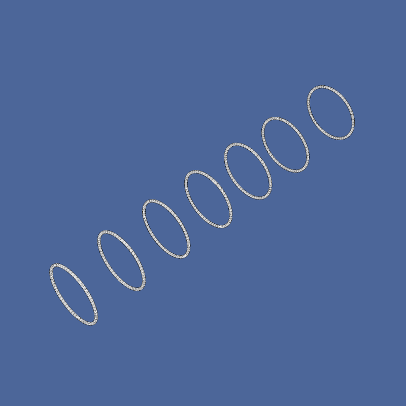
In this example, we’re going to create a simple solver for the equation above and compute the external field in the Eulerian grid. The vortex ring will translate along it’s axis without deformation, as shown in the sequence below
#include "grid/octree.h"
#include "run.h"
#include "view.h"
#include "acastillo/input_fields/filaments.h"
#include "acastillo/input_fields/draw_filaments.h"
#include "acastillo/filaments/biot-savart.h"
In this example, R=1.0, a=0.05 and the vortex ring is discretized into n_{seg}=64 filaments.
int nseg = 64;
double R = 1.0;
double a = 0.05;
double dtmax = 0.005;
struct vortex_filament ring1;

coord Uinfty = {0., 0., 0.};
The main time loop is defined in run.h.
int minlevel = 4;
int maxlevel = 7;
vector u[];
int main(){
  L0 = 10.0;
  X0 = Y0 = Z0 = -L0 / 2;

  periodic(back);
  periodic(top);
  periodic(right);

  N = 1 << minlevel;
  init_grid(N);
  run();
}
Initial conditions
We consider the space-curve \mathcal{C}_1(\xi,t) is parametrized as function of \phi(\xi,t). At time t=0, \begin{aligned} x_1 &= R\cos(\phi), \quad \\ y_1 &= R\sin(\phi), \quad \\ z_1 &= z_0 \end{aligned}
The curve \mathcal{C}_1(\xi,t) will
be stored as struct vortex_filament which must be released
at the end of the simulation.
event init (t = 0) {
  double dphi = 2*pi/((double)nseg);
  double phi[nseg];
  double a1[nseg];
  double vol1[nseg];
  coord C1[nseg];

  // Define a curve
  for (int i = 0; i < nseg; i++){
    phi[i] = dphi * (double)i;
    C1[i] = (coord) { R * cos(phi[i]), R * sin(phi[i]), -5*L0/8.};
    vol1[i] = pi * sq(a) * R * dphi;
    a1[i] = a;
  }

  // We store the space-curve in a structure
  allocate_vortex_filament_members(&ring1, nseg);
  memcpy(ring1.phi, phi, nseg * sizeof(double));
  memcpy(ring1.C, C1, nseg * sizeof(coord));
  memcpy(ring1.a, a1, nseg * sizeof(double));
  memcpy(ring1.vol, vol1, nseg * sizeof(double));

  local_induced_velocity(&ring1);
  for (int j = 0; j < nseg; j++) {
    ring1.a[j] = sqrt(ring1.vol[j]/(pi*ring1.s[j]));
  }

  view (camera="iso");
  draw_tube_along_curve(ring1.nseg, ring1.C, ring1.a);
  save ("prescribed_curve.png");

  FILE *fp = fopen("curve.txt", "w");
  fclose(fp);
We also initialize the Cartesian grid close to the vortex filament and initialize the velocity field to zero.
scalar dmin[];
for (int i = (maxlevel-minlevel-1); i >= 0; i--){
foreach(){
struct vortex_filament params1;
params1 = ring1;
params1.pcar = (coord){x,y,z};
dmin[] = 0;
dmin[] = (get_min_distance(spatial_period=0, max_distance=4*L0, vortex=¶ms1) < (i+1)*ring1.a[0])*noise();
}
adapt_wavelet ((scalar*){dmin}, (double[]){1e-12}, maxlevel-i, minlevel);
}
foreach(){
foreach_dimension(){
u.x[] = 0.;
}
}
}We release the vortex filaments at the end of the simulation.
event finalize(t = end){
  free_vortex_filament_members(&ring1);
}
A Simple Time Advancing Scheme
Time integration is done in two steps. First, we evaluate the (self-)induced velocity at \vec{x}_c
event evaluate_velocity (i++) {

  memcpy(ring1.Uprev, ring1.U, nseg * sizeof(coord));

  local_induced_velocity(&ring1, Gamma=1.0);
  for (int j = 0; j < nseg; j++) {
    ring1.Uauto[j] = nonlocal_induced_velocity(ring1.C[j], &ring1, Gamma=1.0);
    foreach_dimension(){
      ring1.U[j].x = ring1.Uauto[j].x + ring1.Ulocal[j].x - Uinfty.x;
    }
  }
}
Then, we advect the filament segments using an explicit Adams-Bashforth scheme
event advance_filaments (i++) {
  for (int j = 0; j < nseg; j++) {
    foreach_dimension(){
      ring1.C[j].x += dt*(3.*ring1.U[j].x - ring1.Uprev[j].x)/2.;
    }
  }
}
Finally, we compute the new arch-lenghts and update the core sizes to preserve the total vorticity
event advance_filaments (i++, last) {
  local_induced_velocity(&ring1, Gamma=1.0);
  for (int j = 0; j < nseg; j++) {
    ring1.a[j] = sqrt(ring1.vol[j]/(pi*ring1.s[j]));
  }
  dt = dtnext (dtmax);
}
Outputs
Displacement of the vortex filament
We output the position of the ring at regular intervals
event sequence (t += 5.0){
  char filename[100];
  sprintf(filename, "vortex_ring_%g.png", t);

  view(camera="iso");
  draw_tube_along_curve(ring1.nseg, ring1.C, ring1.a);
  save(filename);
}
and use the following script to create a composite image:
convert test_vortex_ring1/vortex_ring_5.png -transparent "rgb(76, 102, 153)" test_vortex_ring1/vortex_ring_5.png
convert test_vortex_ring1/vortex_ring_10.png -transparent "rgb(76, 102, 153)" test_vortex_ring1/vortex_ring_10.png
convert test_vortex_ring1/vortex_ring_15.png -transparent "rgb(76, 102, 153)" test_vortex_ring1/vortex_ring_15.png
convert test_vortex_ring1/vortex_ring_20.png -transparent "rgb(76, 102, 153)" test_vortex_ring1/vortex_ring_20.png
convert test_vortex_ring1/vortex_ring_25.png -transparent "rgb(76, 102, 153)" test_vortex_ring1/vortex_ring_25.png
convert test_vortex_ring1/vortex_ring_30.png -transparent "rgb(76, 102, 153)" test_vortex_ring1/vortex_ring_30.png

convert test_vortex_ring1/vortex_ring_0.png test_vortex_ring1/vortex_ring_20.png -composite temp_image.png
convert temp_image.png test_vortex_ring1/vortex_ring_5.png -composite temp_image.png
convert temp_image.png test_vortex_ring1/vortex_ring_10.png -composite temp_image.png
convert temp_image.png test_vortex_ring1/vortex_ring_15.png -composite temp_image.png
convert temp_image.png test_vortex_ring1/vortex_ring_20.png -composite temp_image.png
convert temp_image.png test_vortex_ring1/vortex_ring_25.png -composite temp_image.png
convert temp_image.png test_vortex_ring1/vortex_ring_30.png -composite test_vortex_ring1/final_image.png
The solution outside the vortex tube
Vortex filaments are treated as Lagrangian particles and may exist outside the mesh. We may also evaluate the induced velocity at any point \vec{x}\in\mathbb{R}^3.

|

|

|

|

|

|
event slice (t += 5.0){
  foreach(){
    coord p = {x,y,z};
    coord u_BS = nonlocal_induced_velocity(p, &ring1);
    foreach_dimension(){
      u.x[] = u_BS.x - Uinfty.x;
    }
  }
  adapt_wavelet ((scalar*){u}, (double[]){1e-4, 1e-4, 1e-4}, maxlevel, minlevel);
  {
    char filename2[100];
    sprintf(filename2, "axial_velocity_%g.png", t);

    view(camera="left");
    cells(n={1,0,0});
    squares ("u.z", linear = true, spread = -1, n={1,0,0}, min=-0.50, max=0.50, map = cool_warm);
    draw_tube_along_curve(ring1.nseg, ring1.C, ring1.a);
    save(filename2);
  }
}
Time evolution
We may also follow the position of \mathcal{C}_1 and the induced velocities over time,
event final (t += 0.10, t <= 36.0){
  if (pid() == 0){
    FILE *fp = fopen("curve.txt", "a");
    write_filament_state(fp, &ring1);
    fclose(fp);
  }
}
import numpy as np
import matplotlib.pyplot as plt
n = 64
ax = plt.figure()
data = np.loadtxt('curve.txt', delimiter=' ', usecols=[0,4])
plt.plot(data[:,0], data[:,1])
plt.xlabel(r'Time $t$')
plt.ylabel(r'Axial coordinate $z$')
plt.xlim([0,30])
plt.tight_layout()
plt.savefig('plot_z_vs_t.svg')
References
| [castillo2022] |
A. Castillo-Castellanos and S. Le Dizès. Closely spaced co-rotating helical vortices: long-wave instability. Journal of Fluid Mechanics, 946:A10, 2022. [ DOI ] |
| [castillo2021] |
A. Castillo-Castellanos, S. Le Dizès, and E. Durán Venegas. Closely spaced corotating helical vortices: General solutions. Phys. Rev. Fluids, 6:114701, Nov 2021. [ DOI | http ] |
| [duran2019] |
E. Durán Venegas and S. Le Dizès. Generalized helical vortex pairs. Journal of Fluid Mechanics, 865:523–545, 2019. [ DOI ] |