sag.c

The SAG equation

The SAG equation

The SAG equation is a diffusion Fick equation of a specie c: \displaystyle \frac{\partial c}{\partial t} =\nabla^2 c with boundary condition of cristal growth on the substrat \frac{\partial c}{\partial y} = bi\; c on y=0 (bi is a kind of Biot number) and no growth \frac{\partial c}{\partial y} = 0 on y=0 on the mask and far from the wall, there is a constant arrival of species c(x,top)=1, right and left are periodic conditions (periodicity is here a symmetry).

This system can be solved with the reaction–diffusion solver.

#include "grid/multigrid.h"
#include "run.h"
#include "diffusion.h"

#define MAXLEVEL 10
#define MINLEVEL 5

Concentration at time t+dt, t and flux, and some obvious variables

scalar c[],cold[],dc[],flux[],dce[];
double beta,bi,w,tmax,dx,errmax;

The generic time loop needs a timestep. We will store the statistics on the diffusion solvers in mgd.

double dt;
mgstats mgd;

the exact solution without mask

double cexact(double y)
{ double ce;
    ce = (bi*y+1)/(bi*L0+1);
    return ce;
}

Boundary conditions: a given concentration at the top, no reaction on the mask (no flux: \partial c(t)/\partial y=0), a complete reaction on the cristal (|x| < w) \partial c(t)/\partial y = bi\; c(t) this mixed condition is written (c[0,0]-c[bottom])/Delta = bi (c[0,0] + c[bottom])/2

c[top]    =  dirichlet(1);
//c[bottom] = (fabs(x)<w)? neumann(0) :  c[]*(2.-bi*Delta)/(2.+bi*Delta) ;

problem with mixed

c[bottom] = (fabs(x)<w)? neumann(0) : val(_s,0)*(2.-bi*Delta)/(2.+bi*Delta)   ; 
c[right]  =  neumann(0);
c[left]   =  neumann(0);

Parameters

The size of the domain L0.

int main() {
    beta = 1;
    L0 = 10.;
    X0 = -L0/2;
    Y0 = 0;
    N =  256;
    dx = L0/N;
    tmax = 100;
    errmax = 5.e-4;

the chemical Biot number and the width of the mask

    bi = 1.;
    w = 1;
    run();
}

Initial conditions

a constant amount of concentration

event init (i = 0) {
    foreach() {
        c[]=cexact(y);
        cold[]=c[];
        dce[]=0;
    }
    boundary ({c,cold});
}

Time integration

event integration (i++) {

We first set the timestep according to the timing of upcoming events. We choose a maximum timestep of 0.2 which ensures the stability of the reactive terms for this example.

    dt = dtnext (dt);

We use the diffusion solver to advance the system from t to t+dt.

    scalar r[],lambda[];
    foreach() {
        r[] = 0;
        lambda[] = 0;
    }

solving \displaystyle \nabla^2 c^{n+1} + (\lambda -\frac{1}{\Delta t}) c^{n+1} + r +\frac{1}{\Delta t} c^{n}= 0

    mgd = diffusion (c, dt, r = r, beta = lambda);
    
    foreach()
    dc[]=cold[]-c[];
    
    foreach()
    cold[]=c[];
    boundary ({cold});

The flux along y is {\partial c}{\partial y}

    foreach()
    flux[] =  ( c[0,0] - c[0,-1] )/Delta;
    boundary ({flux});

end when converged

    double err= sqrt(normf(dc).max);
    fprintf (stdout," %lf %lf\n",t,sqrt(normf(dc).max));
     if((t>1)&&(err < errmax)) {  fprintf (stdout,"stop convergence \n"); exit(1);}
}

Outputs

Here we create mpeg animations

event movies (i += 3; t <= tmax) { fprintf (stderr, “%g %g”, t, sqrt(normf(dc).max)); foreach() dce[] = c[] -cexact(y); static FILE * fp = popen (“ppm2mpeg > c.mpg”, “w”); output_ppm (dce, fp, spread = 2, linear = true);

static FILE * fp1 = popen (“ppm2mpeg > level.mpg”, “w”); scalar l = dce; foreach() l[] = level; output_ppm (l, fp1, min = MINLEVEL, max = MAXLEVEL, n = 512);

}

print data saves along

event printdata (t +=1;t<=tmax) {
    FILE *  fpx = fopen("cutx.txt", "w");
    FILE *  fpy = fopen("cuty.txt", "w");
    //   static double dx = L0/512;
    for (double x = -L0/2 ; x < L0/2; x += dx){
        double y=x+L0/2;
        fprintf (fpx, "%g %g %g \n",
                 x, interpolate (c, x, 0) , interpolate (flux, x, 0.));
        fprintf (fpy, "%g %g %g \n",
                 y, interpolate (c, 0, y) , interpolate (flux, 0, y));}
    fclose(fpx);
    fclose(fpy);
}

At the end of the simulation, we create snapshot images of the field, in PNG format.

event pictures (t +=1) {
    scalar  dce[];
    foreach()
    dce[] =  c[] -cexact(y);
    boundary ({dce});
    output_ppm (dce, file = "c.png", spread = 2, linear = true);
}

We can now use wavelet adaptation. The function then returns the number of cells refined.

event adapt(i++) {
#if QUADTREE
    astats s = adapt_wavelet ({dce}, (double[]){.001},
                              MAXLEVEL, MINLEVEL);
    fprintf (stderr, "# refined %d cells, coarsened %d cells\n", s.nf, s.nc);
    return s.nf;
#else // Cartesian
    return 0;
#endif
}

Run

Then compile and run:

 rm sag; qcc  -g -O2 -DTRASH=1 -Wall  sag.c -o sag ; ./sag

or better

 make sag.tst;make sag/plots    
 make sag.c.html ; open sag.c.html

Results

compare a cut in x=0, exact solution and computed

 set output 'cuty.png'
 bi=1
 L0=10
 set xlabel "y"
 set key left
 p[:][:]'./cuty.txt'u 1:($2) t 'c'w l,''u 1:3 t'dc/dy' w l,bi/(bi*L0+1.) t 'bi/(bi L0+1)',(bi*x+1)/(bi*L0+1) t'(bi y+1)/(bi*L0+1)'

cut in x=0 (script)

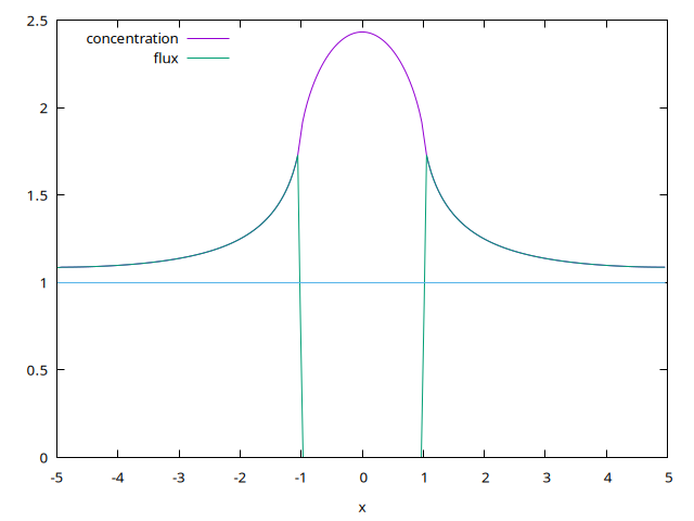
compare a cut in y=0, concentration en flux dived by the reference flux bi/(bi L0+1)

 set output 'cutx.png'
 bi=1
 L0=10
 set xlabel "x"
 p'./cutx.txt'u 1:($2*(bi*L0+1)) t'concentration' w l,''u 1:($3*(bi*L0+1)/bi) t'flux' w l,1 not

cut in y=0 (script)

Field of c:

Bibliography

N. Dupuis, J. Décobert, P.-Y. Lagrée, N. Lagay, D. Carpentier, F. Alexandre (2008): “Demonstration of planar thick InP layers by selective MOVPE”. Journal of Crystal Growth issue 23, 15 November 2008, Pages 4795-4798
N. Dupuis, J. Décobert, P.-Y. Lagrée , N. Lagay, C. Cuisin, F. Poingt, C. Kazmierski, A. Ramdane, A. Ougazzaden (2008): “Mask pattern interference in AlGaInAs MOVPE Selective Area Growth : experimental and modeling analysis”. Journal of Applied Physics 103, 113113 (2008)

Version 1: may 2014, ready for new site 09/05/19