sandbox/Antoonvh/vringinversion.c

An upward travelling vortex ring may be generated by the mt. Etna volcano. Image via tumblr

The interactions of a vortex ring with an inversion layer

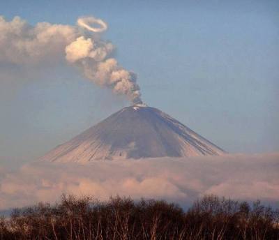
Vortex rings are flow structures that advect trough a fluid. It is therefore very likely that they encouter features on on their trajectories, e.g. an other vortex ring. On this page we study the dynamical behaviour of a vortex ring that ‘collides’ with a sharp intersion layer.

Set-up

For this preliminary study we assume that the evolution of the initially axisymmetric set-up remains axisymmetric, and hence we solve the equations of motion in only two dimenionsions. I.e. with z the axial coordinate and r the distance from the axis of symmetry. The buoyancy inversion is modelled to be infinetly sharp and we track its interface. Gravity is implemented in its ‘reduced’ form. Furthermore, we will view our results.

#include "axi.h"
#include "navier-stokes/centered.h"
#include "two-phase.h"
#include "reduced.h"
#include "view.h"

We define the minor and major radius of the vortex ring and its height relative to the inversion. We set an maximum resolution equivalent to that of a 1024^2-cell equidistant grid.

double zp = -2.5;
double rp = 1.;
double minor = 1./10.;
int maxlevel = 10;
FILE * fpm;
int main(){
  L0 = 7;
  X0 = -5;
  init_grid(1 << 8);

The inversion strength is characteriezed by a relative buoyancy jump (b'), its value can be compared against a measure for the vortex strength, we choose \omega_0^2R, where R is the torus major radius and \omega_0 is the rings’ maximum vorticity for which we assume a Gaussian distribution:

\displaystyle \omega(r)= \omega_0 e^{-r_d^2/\sigma^2}

where \sigma is a typical size of the torus minor radius and r_d the distance from the ring-core centre. Introducing two non-dimensional numbers:

\displaystyle \Pi_1 = \frac{\omega_0^2R}{b'}

\displaystyle \Pi_2 = \frac{R}{\sigma}

From some video footage we guess \omega_0 = \mathcal{O}(1\text{s}^{-1}), R = \mathcal{O}(10\text{m}) and \sigma = \mathcal{O}(1\text{m}). Because these are very rough estimates we will perform runs for a range of b' = \{0.1, 1, 10\}\text{ms}^{-2} corresponding to 0.3K, 3K and 30K inversion strength with a reference potential temperature of 300K. So that \Pi_1 = \{100, 10, 1\}

  rho1 = 1.;
  rho2 = rho1-(rho1/100.);
  mu1 = 1E-7;
  mu2 = mu1;
  fpm = popen("ppm2mp4 movie.mp4", "w");
  G.x = 1.;
  run();
  G.x = 10.;
  run();
  G.x = 100.;
  run();
}

The inversion layer is initialized and a vortex ring is defined with a Gaussian vorticity distribution. We use the \omega \rightarrow \psi \rightarrow \mathbf{u} steps to find the velocity components so that \nabla \cdot \overrightarrow{u} = 0 is automatically statisfied.

event init(i = 0){
  TOLERANCE = 10E-4;
  DT = 10E-4;
  fraction(f, x);
  scalar omega[], psi[];
  psi[bottom] = dirichlet (0.); //The rings' centre is a stream line. 
  refine ((sq(x - zp) + sq(y - rp)) < sq(5*minor) && level < (maxlevel-1));
  refine ((sq(x - zp) + sq(y - rp)) < sq(minor) && level < maxlevel);
  foreach(){
    psi[] = 0.;
    omega[] = exp (-(sq(x - zp) + sq(y - rp))/sq(minor));
  }
  boundary({omega});
  poisson(psi, omega);
  boundary({psi});
  foreach(){
    u.x[] = -(psi[0,1] - psi[0,-1])/(2*Delta);
    u.y[] = (psi[1] - psi[-1])/(2*Delta);
  }
  boundary(all);
}

event adapt(i++){
  DT = min(0.1, DT*1.005);
  adapt_wavelet((scalar*){f,u}, (double[]){0.001, 0.001, 0.001}, maxlevel);
}

Output

We generate movies of our experiments that show the vorticity field (diverging colour map), the interface of the inversion layer (A magenta line) and the used grid (cells).

event bviewer(t += 2. ; t <= 750){
  scalar omega[], psi[];
  char str[99];
  sprintf(str, "Pi_1 = %g", 100/(G.x));
  vorticity(u, omega);
  boundary({omega});
  clear();
  double ang = -M_PI/2.;
  view(fov = 17, psi = ang, ty = 0.25, width = 900, height = 450);
  squares("omega", map = cool_warm);
  draw_vof("f", lc = {1, 0.0, 0.5}, lw = 3);
  mirror({0,-1}){
    cells();
  }
  draw_string(str, size = 40, lw = 3);
  save(fp = fpm);
}

Result

The results are visual:

The dynamics from the last experiment seem to correspond to a ring-collision with a wall / mirror.