sandbox/Antoonvh/primes3D.c

An example Z-order indexing curve of size 4^3, the structure is also known as a Morton Curve. Image courtesy of Asger Hoedt

The prime numbers allong a Z-order space-filling curve, in Three Dimensions

Inspired by Ulam’s spiral and the results that were obtained in two dimensions (2D), it seems atractive to extend the analysis of the locations of the prime numbers (primes) along a Z-order space filling curve to 3D. Convieniently, Basilisk also includes a 3D grid that is iterated in a Z-ordering fashion, namely the Octree grid.

The set-up

The code is copied from the 2D analysis and required only slight alterations. Well done everything that ensures a proper distinction between 2D and 3D grids in the source code! Hence this page only adress the differences in the set-up and results.

#define BV 1 // For Bview movie output 
#include "grid/octree.h"
#include "utils.h"
#include "tag.h"
#if BV
#include "view.h"
#endif

Because of 3D scaling reasons, we can only go to 6 levels of refinement. that corresponds to 2^6=64 points in each direction. We also still use the getprimes function we have used previously on the 2D grid.

int i=6;

void getprimes(int b[],int n){
  b[0]=0;// 0 is not prime
  b[1]=0;// 1 is not prime
  for (int j=2;j<n;j++){
    b[j]=j;
  }
  int j=2;
  while(j<=ceil(sqrt(n))){
    int num = b[j];
    if (b[j]!=0){
      int ind = 2*num;
      while (ind<=n){
	b[ind]=0;
	ind+=num;
      }
    }
    j++;
  }
}

int main(){
  char name[100];
  FILE * fp2 = fopen("connectedregions3d","w");

In 3D, the {x,y,z}={0,0,0} coordinates get centred so that the field-of-view in Bview behaves as expected. The tagging and analysis does not require and modification from the user side to upgrade to 3D, compared to 2D.

  X0=Y0=Z0=-L0/2;
  for (int maxlevel=1;maxlevel<=i;maxlevel++){  
    init_grid(1<<maxlevel);
    scalar field[];
    int d[1<<(maxlevel*dimension)];
    getprimes(d,1<<(maxlevel*dimension));
    int m=1;
    foreach()
      field[]=d[m++];
    int am = tag(field);
    int regsize[am];
    for (m=0;m<am;m++)
      regsize[m]=0;
    foreach()
      if (field[]>0)
	regsize[(int)field[]]++;
    sprintf(name,"prime3d%d.dat",maxlevel);
    FILE * fp = fopen (name, "w");

Output

The output is again similar to what was done in 2D.

1. We store the size of each connected region, for each refinement iteration in seperate files.
2. We store the number of connected regions for each refinement iteration in a single file.
3. A movie is rendered to provide some visual reference.

    for (m=1;m<am;m++)
      fprintf(fp,"%d\n",regsize[m]);
    fprintf(fp2,"%d\t%d\n",maxlevel,am);
    
# if BV //Render a movie
    if (maxlevel==i){
      coord nn ={0,0,1};
      static FILE * fp6 = popen ("ppm2mp4 movie.mp4", "w");
      for (int g=0;g<=pow(2,maxlevel+2);g++){
	double a = ((double)g/pow(2,maxlevel+2))-L0/2.;
	view(fov=30,width=512,height=512,tx=-0.,ty=-0.,theta=0.5,phi=0.5);
	squares("field",map=gray,min=0,max=1,alpha=a,n=nn);
	save (fp = fp6);
	clear();
      }
    }
#endif
  }
}

Results

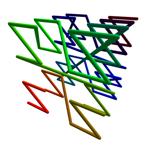
The movie reveals the locations of the primes.

The video clearly shows all-black slices in the domain that give the movie a trippy appearance. These slices corresond to the even numbers that, be design of the natural numbers, account for half of the cells. We also saw these even numbers as lines in the 2D analysis, where they caused connected regions to only extend in the x-direction. Due to our increased dimensionality we now can have connected regions extending in both x and y directions. We will see how this affects the statistics of the length of the connected regions of the highest-resolution grid. This 64^3-grids holds the same primes as the 512^2-grid we have used in the 2D analysis.

   
reset
set key box 
set border 3
file='prime3d6.dat'
binwidth=1
bin(x,width)=width*floor(x/width)

set table "data"

plot file using (bin($1,binwidth)):(1.0) smooth freq with boxes


unset table

set boxwidth 1
set logscale y
set yrange [0.1:20000]
set xlabel 'Length of connected region' 
set ylabel 'Frequency' 
plot "data" index 0 using ($1):($2) with boxes title 'Freqency',\
  5000*exp(-0.5*x) t 'e^{x/2} scaling ' lw 3 ,\
 100000*exp(-2*x) t 'Scaling from the 2D analysis' lw 3 

Histogram of the length of the connected regions. (script)

The connected regions are more frequently longer compared to the 2D scaling behaviour. Consequently, we observe that the extra dimension gave rise to different scaling behaviour.

Next we check if this has also affected the scaling of the number of connected regions with further extending grids.

 reset
 set xr[0.5:6.5]
 set xlabel 'Refinement level'
 set ylabel 'Number of connected regeons'
 set logscale y
 set key box bottom right
 set size square
 plot 'connectedregions3d' using 1:2 title 'Number of connected regions',\
 0.04*2**(2.85*x) with lines title '2.85-Dimensional scaling' lw 3 ,\
 0.1*2**(1.9*x) with lines title '1.9-Dimensional scaling from the 2D grid' lw 3

(script)

I think this result is not too surprising now, given that maybe in 1D the number of primes aproximates the number of regions and that scales with 0.95 N, where N is the number of cells. Than the corresponding scaling behaviour in higher dimensions (D) is just 0.95 \times D, because that is how much more grid cells there are in higher dimensions with increasing refinement.