bomex.c

Shallow cumulus convection

Shallow cumulus convection may brighten your day! Image by Hongbin Chen via phys.org

Shallow cumulus convection

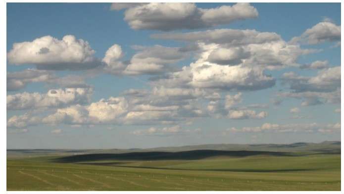
Since the spring is upon us we hope to see a bunch of fair-weather clouds soon. For the time being we will simulate them.

Set-up

We follow the seminal BOMEX scenario formulated in Siebesma et. al. (2002). Notice that we implement a two-dimensional analogy here. The setup is chosen such that there exist a conditionally unstable region in the atmosphere. It is an important ingredient for vertical momentum transport in the atmosphere. We rely on the formulations under thermo.h.

#include "navier-stokes/centered.h"

We solve the equations of motion in a moving frame of reference.

double U_TRANS = -4;
#define U_GEO ((y < 700 ? -8.75 : -8.75 + (-4.61 - -8.75)*(y - 700)/(3000 - 700)) - U_TRANS)
#include "force_geo.h"
#include "thermo.h"

Periodic boundaries are set and we use a 6 km domain in all directions.

int main() {
  periodic (left);
#if dimension > 2   
  periodic (front);
#endif
  L0 = 6000.;
  run();
}

The case is defined by forcings and large-scale tendencies (which we forget), and the initial vertical profiles:

event init (t = 0) {
  f_cor = 0.376e-4;
  T_ref = 300; //Reference temperature
  P0 = 101500; //Surface pressure
  foreach() {
    u.x[] = U_GEO;
    thl[] = (y < 520 ? 298.7 :
	     y < 1480 ? 298.7 + (302.4 - 298.7)*(y - 520)/(1480 - 520) :
	     y < 2000 ? 302.4 + (308.2 - 302.4)*(y - 1480)/(2000 - 1480) :
	     308.85 + (311.85 - 308.2)*(y - 2000)/(3000 - 2000));
    qt[] = (y < 520 ? 17. + (16.3 - 17.)*y/(520) :
	    y < 1480 ? 16.3 + (10.7 - 16.3)*(y - 520)/(1480 - 520) :
	    y < 2000 ? 10.7 + (4.2 - 10.7)*(y - 1480)/(2000 - 1480) :
	    4.2 + (3. - 4.2)*(y - 2000)/(3000 - 2000))*1e-3;
    u.y[] += 0.01*noise()*exp(-y/500.); 
  }
  boundary (all);
  set_pres (guess = true);
  scalar pt[];
  do {
    set_pres();
  } while (change (pres, pt) > 0.01);
  boundary ({pres});
}

At the top boundary, the profiles follow the prevailing gradient.

thl[top] = neumann((311.85 - 308.2)/1000.);
qt[top] = neumann((3 - 4.2)*1e-3/1000.);
u.t[top] = neumann((-4.61 - -8.75)/2300.);

The computation of the surface fluxes are simple and described by the case setup.

event surface_fluxes (i++) {
  foreach_boundary(bottom) {
    qt[]  += dt*5.2e-5/Delta;
    thl[] += dt*8e-3/Delta;
    u.x[] -= (dt*sq(0.28)*(u.x[] + U_TRANS)/
	      (sqrt(sq(u.x[] + U_TRANS) + sq(uz[]))))/Delta;
    uz[]  -= (dt*sq(0.28)*uz[]/
	      (sqrt(sq(u.x[] + U_TRANS) + sq(uz[]))))/Delta;
  }
}

Grid adaptation

The grid is adapted to accurately represent the total water specific humidity, the liquid water potential temperature and the velocity components. The resolution varies between ca. 187 m and 25 m.

event adapt (i = 5 ; i++) 
  adapt_wavelet ((scalar*){qt, thl, u},
		 (double[]){0.002, .5, 0.125, 0.125, 0.125}, 8, 5);

The simulation stops after two hours

event stop (t = 2*3600);

Output

We generate simple movies showing the evolution of The cloud-water specific humidity (q_c):

Clouds!

The liquid water potential temperature \theta_l:

And the grid resolution:

Redder is better

We also plot some all-important vertical profiles, taken at t = 1h:

set yr [0:2500]
set xlabel 'Specific humidity'
set ylabel 'height'
plot 'profiles' u 5:1 w l lw 2 t 'Total', 'profiles' u 6:1 w l lw 2 t 'Cloud'

(script)

set key off
set xlabel 'Potental temperature (liquid water)
plot 'profiles' u 4:1 w l lw 2

(script)

set xlabel 'Horizontal velocity'
plot 'profiles' u 2:1 w l lw 2 t 'u.x', 'profiles' u 3:1 w l lw 2 t 'uz'

(script)

event write_profile (t = 3600) {
  scalar qc[], uh[];
  foreach() {
    uh[] = u.x[] + U_TRANS;
    qc[] = QC;
  }
#if dimension == 2
  profile ({uh, uz, thl, qt, qc}, fname = "profiles");
#endif
}	       

event dumper (i += 200) {
  char fname[99];
  sprintf(fname, "dump%d", i);
  dump (fname);
}

event movie (t += 30) {
  scalar qc[], lev[];
  foreach() {
    qc[] = QC;
    lev[] = level;
  }
  output_ppm (thl, file = "thl.mp4", n = 512,
	      min = 298.5, max = 302, box = {{0,0},{L0,L0/2}});
  output_ppm (qc, file = "qc.mp4", n = 512, min = 0, max = 0.002,
	      map = cloud, box = {{0,0},{L0,L0/2}} );
  output_ppm (lev, file = "level.mp4", n = 512,
	      min = 4, max = grid->maxdepth);
}

Reference

Siebesma, A. Pier, et al. “A large eddy simulation intercomparison study of shallow cumulus convection.” Journal of the Atmospheric Sciences 60.10 (2003): 1201-1219.