/**
# $2^{\text{nd}}$ Order Interpolation at Resolution Boundaries
On this page i report my motivation and findings regarding the implementation of a higher order interpolation strategies when defining ghost values at resolution boundaries. I.e. for both restriction and prolongation. Notice that a lot of the claims on this page are nonsense.
## Short Intro
Many numerical schemes in basilisk are second order accurate. However, the default treatment of resolution boundaries when using tree grids is only first order accurate. As such, resolution boundaries can become a relevant source of errros under some conditions. A higher order interpolation method could help tackle this challenge.
## Long Introduction
The tree grid facilitates a convienient handling for anisotropic grids by introducing hirarchy in the grid resolution in terms of so-called levels. At some locations this means that leaf cells at different levels appear as neigbors, this is what we refer to as a resolution boundary. Note that neigbors, as referred to in the basilisk code, are always at the same level and this is the definition that will be used in the rest of this text. Thus leaf cells at resolution boundaries are not neighbors. By design leaf cells at resolution boundaries always differ one level of refinement and accordingly the spatial resolution differs a factor of two. In order to handle such a jump in resolution two types of (ghost) cells are introduced.
* Restriction: The parent cell of the fine cell(s) at the resolution boundary (i.e. at one level lower) gets a value assigned by the restriction operation. For example, the coarse level value is determined by avereging the values of all its children. Note that restriction is performed for all coarse level (non leaf parent) cells in order to apply multigrid schemes. As such i believe it is formally not reffered to as a ghost cell.
* Prolongation or Halo cells: The children of the coarse leaf cell at a resolution boundary are initialized (i.e. said to be active cells). The values used are defined by the prolongation operation. For example, by linear interpolation using the original cell and its neighbors' values.
Using this method, all leaf cells at resolution boundaries have defined neigbors and this facilitates the usage of the more general multigrid methods to be extended to the tree based grid. Unfortunately, the interpolation methods used for restriction and prolongation are not exact and therefore introduce errors at the locations of resolution boundaries.
When using adaptive grids the wavelet estimated error adaptive algorithm (wavelet algorithm) is a power full tool to access the required variable level of refinement required within the domain. It can be viewed as an assessment of what error the interpolation technique would introduce and if this is within a certain set limit (the refinement criterion). An imperfect feature of this method is that whenever it decides the introduce a resolution boundary a fraction of the maximum tolerated error is actually introduced! Thereupon it is common practice to limit the maximum resolution to a pre-defined value. This way, a small refinement criterion can be chosen such that the introduced interpolation errors at resoltion boundaries are small whilst limiting the "Overeagerness" of the refinement algorithm when using this small value. This works really well. However, (personally) i identify two challenges such a strategy poses.
* Apart from finding a suitable refinement criterion, the user is burdened with defining a suitable maximum resolution.
* Adaptive grids are the method of choice to study the interplay of different physical mechanisms that occur at different length and time scales. But the inherent "overeagerness" of the algorithm as described above tends to overresolve the processes that do not require the maximum resolution.
The last point can be a bit vague. Therefore i have uploaded an [example case](lamb-dipole.c) of a such a multi process physical system based on the collision of a dipolar vortex with a no slipp wall. For high reynolds numbers the correct resolving the boundary layer at the no-slip wall requires a much higher resolution compared to resolving the advection of the initial dipole. This is due to the much smaller curvature in the solution at the dipole compared to the induced boundary layer. The wavelet algorithm is able to pick this up correctly but because i need to limit interpolation errors it starts to over resolve the inital dipole approach, leading to a reduced computational efficientcy. This reduced efficientcy can grow out of hand if the interpolation errors do not scale favourably when introducing more resolution boundaries.
## Qualitative Analysis using the default Basilisk settings
We bases our analysis on the diffusion of a 1D gaussian plume and focus on the bahaviour or the errors using a wavelet algorithm based grid. We do not limit the maximum level, as we act as if this problem is part of a larger system that requires us to use a higher maximum resolution. Furthermore, we focus on a very short time span such that we can use a very small timestepping and we do not need to adaptively to change the grid. This ensures that there are no appricable erros due to the time intetgration scheme. Additionally the tolerance for the poisson solver is also set to a small value. As such, all errors should be due to the spatial discretization. Note that these are actually not the default settings of Basilisk. In the chosen time span the peak value of the gaussian pulse drops to $\approx 90\%$ of the initialized value. The used code is as follows:
*/
#include "grid/bitree.h"
#include "run.h"
#include "diffusion.h"
scalar A[];
mgstats mgA;
double vis = 0.03, Ae=0.00125;
scalar err[];
scalar r[],rc[];
int maxlevel = 15;
const face vector diff[] = {vis,vis};
int main()
{
L0 = 25;
X0=Y0=-L0/2;
init_grid(1<<(7));
run();
}
event init(i=0)
{
int tot = 1, it =0;
TOLERANCE=1e-10;
double tz = 1/(4*vis)-(4);
fprintf(ferr,"tz = %g\n",tz);
DT=0.0005;
foreach()
{
rc[] = pow((pow(x,2)+pow(y,2)),0.5);
A[]= exp((-(pow(rc[],2)))/(4*vis*tz));
}
boundary(all);
while (tot>0)
{
it++;
fprintf(ferr,"iteration %d of adapt wavelet\n",it);
astats f = adapt_wavelet({A},(double[]){Ae},maxlevel,4,{A});
foreach(){
rc[] = pow((pow(x,2)+pow(y,2)),0.5);
A[]= exp((-(pow(rc[],2)))/(4*vis*tz));
}
boundary({A});
tot = f.nf+f.nc;
fprintf(ferr,"%d\t",tot);
}
fprintf(ferr,"\nIt took %d iterations of the 'adapt-wavelet' function to initialize the field\n",it);
int l=0;
int n=0;
foreach(){
n++;
if (level>l)
l=level;
}
fprintf(ferr,"max level = %d, cells = %d\n",l,n);
dt=DT;
}
event output (t+=0.01)
{
double tz = 1/(4*vis)-(4);
double error = 0;
fprintf(ferr,"t=%g\t",t);
foreach(reduction(+:error))
{
err[]=fabs(A[]-( pow(tz/(tz+t),0.5)) * exp((-(pow(x,2)+pow(y,2)))/(4*vis*(tz+t))));
error+=err[]*Delta;
}
fprintf(ferr,"error = %g \n" ,error);
}
event stop (t=1)
{
foreach()
fprintf(ferr,"%f\t%d\t%g\t%g\n",x,level,err[],A[]);
}
event Diffusion (i++;t<=1)
{
dt = dtnext (t,DT);
mgA=diffusion(A,dt,diff);
boundary(all);
}
/**
The results are as follows:
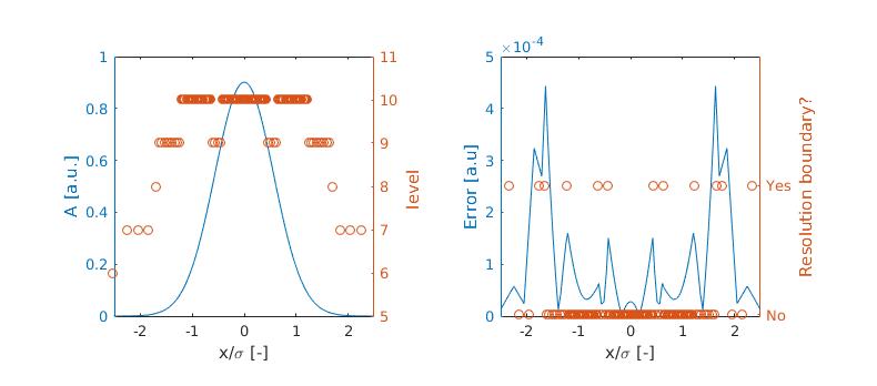
It is clear that the error compared to the analytical solution peaks at the location of resolution boundaries and appears to leak (diffuse) into the other grid cells as well. This forms a base line for the following analysis. It should be noted however that the wavelet algorithm did do a great job of refining and coarsening the grid such that the errors are now more evenly distributed troughout the domain eventough the resolution varies several levels! We keep this in mind when we arrive at the conclusions (if ever).
## Method
In order to limit the errors due to the interpolation strategy for prolongation and restriction it could be beneficial to base it on a higher order strategy. By default restriction of a scalar is a simple averaging of the children values and prolongation uses a linear interpolation as was used as example in the introduction. Such methods are only first order accurate. Meaning that such a method is exact when the solution is constant or a linear function in space. One order higher up we arrive at so-called second order accurate techniques. These are able to exactly capture quadratic curvature in a solution field. If this was the end of the story restriction and prolongation would look something like this,
For restriction / coarsening:
*/
static inline void coarsen_quadratic (Point point, scalar s)
{
double sum = 0.;
#if dimension == 1
foreach_child()
sum += 9*s[]-s[child.x,0,0];
s[] = sum/(16);
#elif dimension==2
foreach_child()
sum += 10*s[]-s[child.x,0,0]-s[0,child.y,0];
s[] = sum/(32);
#else //dimension ==3
foreach_child()
sum += 11*s[]-s[child.x,0,0]-s[0,child.y,0]-s[0,0,child.z];
s[] = sum/(64);
#endif
}
/**
and for prolongation / refine:
*/
static inline void refine_quadratic (Point point, scalar s)
{
#if dimension == 1
foreach_child()
s[]=(30*coarse(s,0)+5*coarse(s,child.x)-3*coarse(s,-child.x))/32;
#elif dimension == 2
foreach_child()
s[]=(296.*coarse(s,0,0) +5.*coarse(s,child.x,child.y) +
146.*(coarse(s,child.x,0) + coarse(s,0,child.y)) +
98.*(coarse(s,-child.x, 0) + coarse(s,0,-child.y)) -
61.*(coarse(s,child.x,-child.y) + coarse(s,-child.x,child.y))-
91.*(coarse(s,-child.x,-child.y)))/576.;
#else //dimension == 3
foreach_child()
s[]=(412*coarse(s,0,0)+
262.*(coarse(s,child.x,0,0)+coarse(s,0,child.y,0)+coarse(s,0,0,child.z))+
121.*(coarse(s,child.x,child.y,0)+coarse(s,child.x,0,child.z)+
coarse(s,0,child.y,child.z))+
214.*(coarse(s,-child.x,0,0)+coarse(s,0,-child.y,0)+coarse(s,0,0,-child.z))-
11.*(coarse(s,child.x,child.y,child.z))+
55.*(coarse(s,child.x,-child.y,0)+coarse(s,-child.x,child.y,0)+
coarse(s,child.x,0,-child.z)+coarse(s,-child.x,0,child.z)+
coarse(s,0,child.y,-child.z)+coarse(s,0,-child.y,child.z))-
95.*(coarse(s,child.x,child.y,-child.z)+coarse(s,child.x,-child.y,child.z)+
coarse(s,-child.x,child.y,child.z))+
25.*(coarse(s,-child.x,0,-child.z)+coarse(s,0,-child.y,-child.z)+
coarse(s,-child.x,-child.y,0))-
143.*(coarse(s,-child.x,-child.y,child.z)+coarse(s,-child.x,child.y,-child.z)+
coarse(s,child.x,-child.y,-child.z))-
155.*coarse(s,-child.x,-child.y,-child.z))/1728;
#endif
}
/**
The weights are based on the linear regression of the second order accurate function in a given dimension to the cell in question and all it neighbors' values. i.e.
$$ f(x)=ax^2+bx+c,$$
$$ f(x,y)=ax^2+by^2+cxy+dx+fy+g,$$
$$ f(x,y,z)=ax^2+by^2+cz^2+dxy+exz+fyz+gx+hy+iz+jd,$$
in 1,2 or 3 dimensions, respectively.
Because the restriction operation does now require values outside the parent cell (that gets restricted) it does not work at resolution boundaries. You would need the prolongated value for this. However those are typically not defined before we have done the restriction because of a similar reasoning.
A possible solution is to base the second order restriction on leaf cells only. And here i have tried to do this using the following method, currently only defined for one dimensional problems:
This requires separate interpolation functions for the tree different case of where the non-leaf neighbors are located (left, right or both). Those are called according to the following coarsening strategy:
*/
static inline void quadratic_boundary_restriction(Point point, scalar s)
{
if (!is_leaf(neighbor(-1)&&!is_leaf(neighbor(1))))
coarsen_average(point, s);// We maintain the regular averaging if the cell is not part of a resolution boundary.
// coarsen_quadratic(point, s); // but inprinciple we cloud choose otherwise.
else if (is_leaf(neighbor(-1))&&is_leaf(neighbor(1))) // At coarse level l, both neighbors are leafs
coarsen_twoleaf_quad(point,s);
else if (is_leaf(neighbor(-1))&&!is_leaf(neighbor(1))) // Only left left neighor is a leaf
coarsen_leftleaf_quad(point,s);
else if (!is_leaf(neighbor(-1))&&is_leaf(neighbor(1))) // Only right hand side neighbor is a leaf
coarsen_rightleaf_quad(point,s);
}
/**
and are defined as follows:
*/
static inline void coarsen_twoleaf_quad (Point point, scalar s)
{
assert(dimension==1);
double sum = 0.;
foreach_child()
sum += 16*s[];
sum+=-(s[-1]+s[1]);
s[] = sum/(30);
}
static inline void coarsen_leftleaf_quad (Point point, scalar s)
{
assert(dimension==1);
double sum = 0.;
foreach_child(){
if (child.x==-1)
sum += 591.2*s[];
else
sum+=(((490.5*s[])+(-32.3*s[child.x])));
}
sum+=-49.4*(s[-1]);
s[] = sum/(1000);
}
static inline void coarsen_rightleaf_quad (Point point, scalar s)
{
assert(dimension==1);
double sum = 0.;
foreach_child(){
if (child.x==1)
sum += 591.2*s[];
else
sum+=(((490.5*s[])+(-32.3*s[child.x])));
}
sum+=-49.4*(s[1]);
s[] = sum/(1000);
}
/**
Again the weights are found by linear regression of the functions mentioned earlier, now evaluated to values on the non-equidistant grid of leafs.
By adding the code above to "src/grid/multigrid-common.h" we can set the coarsening and prolongation attribute for scalar A to employ our method.
*/
...
A.coarsen=coarsen_boundary_restriction;
A.prolongation=refine_quadratic
boundary({A});
....
/**
Note that in the example if the 1D Gaussian pulse, this should be added after we have based our grid on the wavelet algorithm since we are happy with the default coarsening when it comes to estimating errors. Remember that I only want to alter the interpolation strategy during computations. Currently these fundamentally different procedures are "hard-coded" to be one and the same. Note that for prolongation we do not need to define a cumbersome strategy because these are defined from the bottom up (low to high level) after the restriction procedure has been completed. Therefore, all parents to halo/prolongation ghost children will have leaf neighbors or neigbors that have values defined by second order accurate coarsening and/or prolongation.
## Results
The Results of such a strategy can be compared to the default formulation. The new error field is shown below:
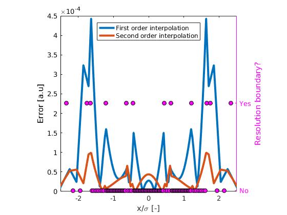
We see that in general the error are substantially smaller. At some resolution boundaries errors seem to be minimal! However, at $x\approx\pm0.7$ the errors remain the same. This can be exaplained by the fact that here there is limited benefit from the higher order interpolation strategy. This is due to the fact that the taylor expansion of the solution at this location does not have a large second order contribution. Furthermore, in the center we see an increased error. I can only explain this with the fact that the errors caused by the 1st interpolation have a different sign than the errors due to the other numerical schemes. Therefore, they can have a compensating effect under some conditions.
The simulation did slow down by approximately 10%
Using -DTRACE=2 when compiling and using the default settings (first order) i got:
*/
# Binary-tree, 2002 steps, 0.515717 CPU, 0.5157 real, 5.28e+05 points.step/s, 8 var
calls total self % total function
2002 0.51 0.47 90.6% Diffusion():diffusionsta1D.c:88
16309 0.04 0.04 8.0% boundary():/home/antoon/basilisk/src/grid/cartesian-common.h:273
101 0.01 0.01 1.0% output():diffusionsta1D.c:76
2 0.00 0.00 0.2% stop():diffusionsta1D.c:82
1 0.52 0.00 0.1% run():/home/antoon/basilisk/src/run.h:39
1 0.00 0.00 0.1% init():diffusionsta1D.c:62
2 0.00 0.00 0.0% init_grid():/home/antoon/basilisk/src/grid/tree.h:1624
14 0.00 0.00 0.0% boundary():/home/antoon/basilisk/src/grid/cartesian-common.h:263
/**
With second order interpolation at resolution boundaries i got:
*/
# Binary-tree, 2002 steps, 0.550729 CPU, 0.5507 real, 4.94e+05 points.step/s, 8 var
calls total self % total function
2002 0.55 0.51 90.9% Diffusion():diffusionsta1D.c:88
16289 0.04 0.04 7.9% boundary():/home/antoon/basilisk/src/grid/cartesian-common.h:273
101 0.00 0.00 0.9% output():diffusionsta1D.c:76
2 0.00 0.00 0.2% stop():diffusionsta1D.c:82
1 0.56 0.00 0.1% run():/home/antoon/basilisk/src/run.h:39
1 0.00 0.00 0.1% init():diffusionsta1D.c:62
2 0.00 0.00 0.0% init_grid():/home/antoon/basilisk/src/grid/tree.h:1624
14 0.00 0.00 0.0% boundary():/home/antoon/basilisk/src/grid/cartesian-common.h:263
/**
The slowing down appears be caused by the additional time spend in the diffusion routine. I expect that the possion solver does requires some additional effort to come to a converged solution.
*/