src/test/viscous.c

Viscous dissipation of a linear wave

Using the multilayer model, we try to reproduce the prediction of Lamb (1932) that the total energy of a small amplitude (linear) water wave should decrease like E(t) = E_0 \exp(-4 \nu k^2 t) with \nu the kinematic viscosity and k the wavenumber.

Joseph & Wang (2004) also showed that if a free-slip rather than a free-surface stress-free condition at the top is applied, one gets instead E(t) = E_0 \exp(-2 \nu k^2 t)

We get the following figure, where the numerical results have been checked for numerical convergence. The numerics clearly agree better with Joseph & Wang than with Lamb.

set xlabel 't/T_0'
set ylabel 'Normalised energy E/E_0'
k = 2.*pi
nu = 1./20000.
lambda = 1.
g = 1.
T0 = k*lambda/sqrt(g*k)
set xrange [0:10]
plot 'log' u ($1/T0):4 every 30 w p t 'Numerical', \
     exp(-2.*nu*k**2*x*T0) w l t 'Joseph and Wang', \
     exp(-4.*nu*k**2*x*T0) w l t 'Lamb'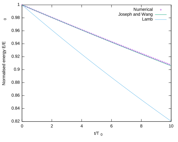

References

See also

• Equivalent case with the Navier-Stokes solver

#include "grid/multigrid1D.h"
#include "layered/hydro.h"
#include "layered/nh.h"
#include "layered/remap.h"
#include "layered/perfs.h"

We reuse the Stokes wave initialisation routine for simplicity. The nonlinear Stokes terms do not matter since the amplitude is small, although this could be checked by using a pure linear wave solution.

#include "test/stokes.h"

The wavenumber is k=2\pi, the amplitude/slope ak is small enough (decreasing it has little effect on the results). The viscosity is \nu=1./RE. Decreasing the viscosity (or increasing it) does not affect the results qualitatively.

Note that we set the fluid depth to h_ = 2 (i.e. twice the wavelength) to be in the deep water limit. This is important to match the theory. Further increasing the depth does not change the results.

double k_ = 2.*pi, h_ = 2., g_ = 1., ak = 0.01;
double RE = 20000.;

This is the wave period.

#define T0  (k_*L0/sqrt(g_*k_))

int main()
{
  periodic (right);
  G = g_;
  nu = 1./RE;

We adjust the numerical parameters for convergence. The vertical resolution matters, as do the convergence of the multigrid solver and timestep. The values below are converged i.e. increasing N, nl and NITERMIN or decreasing DT has little effect on the results.

  N = 256;
  nl = 60;
  NITERMIN = 3;
  DT = 1e-2 [0,1];
  
  run();
}

We optimise layers using a geometric distribution to better resolve the surface, and initialize the wave height and velocity components.

event init (i = 0)
{
  geometric_beta (1./3., true);
  
  foreach() {
    zb[] = - h_;
    double H = wave(x, 0) - zb[];
    double z = zb[];
    foreach_layer() {
      h[] = H/nl;
      z += h[]/2.;
      u.x[] = u_x(x, z);
      w[] = u_y(x, z);
      z += h[]/2.;
    }
  }
}

We need to add the horizontal viscosity. This is important.

event viscous_term (i++) {
  horizontal_diffusion ({u, w}, nu, dt);
}

We plot some free surface profiles, as a visual check. We only do 10 wave periods. This is largely sufficient to measure dissipation.

This confirms that the wave evolution matches the theoretical wave period. The decrease in amplitude is also visible.

set xlabel 'x'
set ylabel 'z'
set xrange [0:1]
plot 'out' w l t ''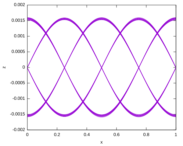

event profiles (t += T0/4.; t <= 10.*T0) {
  foreach (serial) {
    double H = zb[];
    foreach_layer()
      H += h[];
    printf ("%g %g\n", x, H);
  }
  printf ("\n\n");
}

We compute and log the kinetic, potential and total (normalised) energies. The initial condition seems to lead to an initial “jump” (i.e. relaxation) in the numerical solution, so we skip the first timestep. This may be improved.

event logfile (i = 1; i++)
{
  double ke = 0., gpe = 0.;
  foreach (reduction(+:ke) reduction(+:gpe)) {
    double zc = zb[];
    foreach_layer() {
      double norm2 = sq(w[]);
      foreach_dimension()
	norm2 += sq(u.x[]);
      ke += norm2*h[]*dv();
      gpe += (zc + h[]/2.)*h[]*dv();
      zc += h[];
    }
  }
  double Ec = ke/2., Ep = g_*(gpe + L0*sq(h_)/2.);
  double E = Ec + Ep;
  static double E0 = 0.;
  if (i == 1)
    E0 = E;  
  fprintf (stderr, "%g %g %g %g\n", t, Ec, Ep, E/E0);
}