src/test/viscous-ns.c

Viscous dissipation of a linear wave

This is the “Navier–Stokes” equivalent of the multilayer version, which should be consulted for more context.

We solve the two-phase Navier–Stokes equations using a momentum-conserving transport of each phase. Gravity is taken into account using the “reduced gravity approach”.

The viscous decay of the total energy follows Lamb’s prediction (1932) and not Joseph & Wang (2004), in contrast with the multilayer formulation. This reflects the differences in the way the free-surface or interfacial stress conditions are represented in the two approaches.

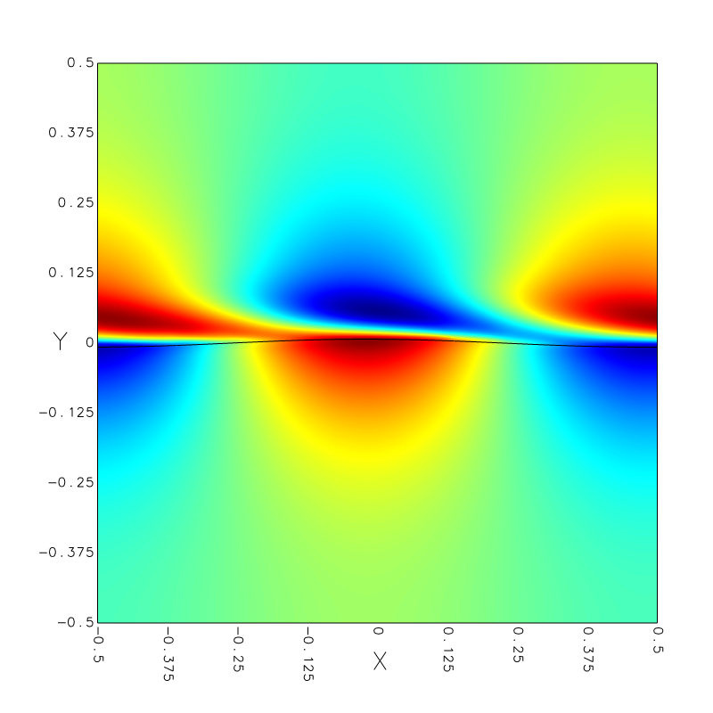
Note that the oscillations in the energy are due to the fact that the initial condition we impose is very “rough” because it does not verify the two-phase equations we are solving here (the initial velocity in the gas is set to zero). The code adjusts this incorrect initial condition in an initial transient (~ 5 timesteps), but the full solution is complex, with the development of boundary layers in both the liquid and gas as shown in the figure below.

set xlabel 't/T_0'
set ylabel 'Normalised energy E/E_0'
k = 2.*pi
nu = 1./20000.
lambda = 1.
g = 1.
T0 = k*lambda/sqrt(g*k)
set xrange [0:10]
plot 'log' u ($1/T0):4 every 30 w p t 'Numerical', \
     exp(-2.*nu*k**2*x*T0) w l t 'Joseph and Wang', \
     exp(-4.*nu*k**2*x*T0) w l t 'Lamb'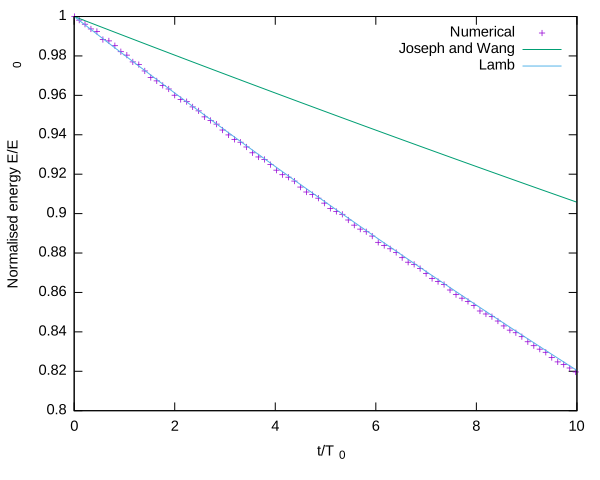

#include "grid/multigrid.h"
#include "navier-stokes/centered.h"
#include "two-phase.h"
#include "navier-stokes/conserving.h"
#include "reduced.h"
#include "test/stokes.h"
#include "view.h"

double k_ = 2.*pi, h_ = 0.5, g_ = 1., ak = 0.05;
double RE = 20000.;
int LEVEL = 8;

The density and viscosity ratios are those of air and water.

#define RATIO (1./850.)
#define MURATIO (17.4e-6/8.9e-4)

T0 is the wave period.

#define T0  (k_*L0/sqrt(g_*k_))

int main ()
{

The domain is a cubic box centered on the origin and of length L0=1, periodic in the x-direction.

  origin (-L0/2, -L0/2);
  periodic (right);

Here we set the densities and viscosities corresponding to the parameters above.

  rho1 = 1. [0];
  rho2 = RATIO;
  mu1 = 1./RE;
  mu2 = 1./RE*MURATIO;
  G.y = -g_;

  N = 1 << LEVEL;
  DT = 1e-2 [0,1];
  run();
}

Initial conditions

This is rough, because we set everything to zero in the gas phase i.e. the initial velocities are discontinuous through the interface etc.

event init (i = 0)
{
  fraction (f, wave(x,y));
  foreach()
    foreach_dimension()
      u.x[] = u_x(x,y)*f[];
}

event profiles (t += T0/4.; t <= 10.*T0) {
  output_facets (f, stdout);
  printf ("\n");
}

We only log after five timesteps to let the numerical transient pass.

event logfile (i = 5; i++)
{
  double ke = 0., gpe = 0.;
  foreach (reduction(+:ke) reduction(+:gpe)) {
    double norm2 = 0.;
    foreach_dimension()
      norm2 += sq(u.x[]);
    ke += norm2*f[]*dv();
    gpe += y*f[]*dv();
  }
  double Ec = ke/2., Ep = g_*(gpe + L0*sq(h_)/2.);
  double E = Ec + Ep;
  static double E0 = 0.;
  if (i == 5)
    E0 = E;  
  fprintf (stderr, "%g %g %g %g\n", t, Ec, Ep, E/E0);
}

event image (t = end)
{
  view (tx = 0.0372524, ty = 0.0235351, tz = -3, bg = {1,1,1});
  draw_vof (c = "f");
  box ();
  squares (color = "u.x", spread = -1, linear = 1);
  save ("u.x.png");
}