sandbox/yixian/granular_bottom_linearisedconstantNGF.c
Flow in a Sandglass / Hourglass / Silo with a bottom orifice
We propose an implementation of the linearised constant non-local granular fluidity(NGF) model for the flow in a silo with a bottom orifice.
Code
Includes and definitions
#include "grid/multigrid.h"
#include "navier-stokes/centered.h"
#include "vof.h"
// Domain extent
#define LDOMAIN 1.
// heap definition
double  H0,R0,D,W,tmax,zetaA;
passive fluid small density to preserve 0 pressure and small viscocity
#define RHOF 1e-4
#define mug  1e-5
// Maximum refinement
#define LEVEL 6
char s[80];
FILE * fpf,*fwq;
scalar f[];
scalar * interfaces = {f};
face vector alphav[];
face vector muv[];
scalar rhov[];
scalar duxx[],duxy[],duyx[],duyy[],dpdx[],dpdy[];

scalar Ifield[],gfield[],gloc_lap[];
scalar eta[];
Boundary conditions
p[top] = dirichlet(0);
pf[top] = dirichlet(0);
u.n[top] = neumann(0);
u.t[bottom] =  fabs(x-LDOMAIN/2)<= W/2 ? neumann(0):  dirichlet(0);
u.n[bottom] =  fabs(x-LDOMAIN/2)<= W/2 ? neumann(0):  dirichlet(0);
p[bottom]   =  fabs(x-LDOMAIN/2)<= W/2 ? dirichlet(0): neumann(0);
pf[bottom]   =  fabs(x-LDOMAIN/2)<= W/2 ? dirichlet(0): neumann(0);
u.n[right] = dirichlet(0);
u.n[left] = dirichlet(0);
u.t[right] = dirichlet(0);
u.t[left] = dirichlet(0);

gfield[left]   = dirichlet(0);
gfield[right]  = dirichlet(0);
gfield[top]    = neumann(0);
gfield[bottom] = fabs(x-LDOMAIN/2)<= W/2 ? neumann(0):  dirichlet(0);


int main(int argc, char ** argv) {

    disable_fpe (FE_DIVBYZERO|FE_INVALID);
    L0 = LDOMAIN;
    // number of grid points
    N = 1 << LEVEL;
    TOLERANCE = 1e-3;
    H0=0.9;
    R0=20.000;

    const face vector g[] = {0.,-1.,0};
    a = g;
    alpha = alphav;
    mu = muv;
    rho=rhov;
    // maximum timestep
    DT = 0.001;
    tmax = 4.;
    W = 0.25;
    zetaA = 0.5;
    D = 0.04375; // Grain size
    fpf = fopen ("interface.txt", "w");
    run();
    fclose (fpf);
    fprintf (stdout,"\n");

}
initial heap, a rectangle
event init (t = 0) {
    scalar phi[];
    foreach_vertex()
    phi[] = min(H0 - y, R0 - x);
    fractions (phi, f);
lithostatic pressure, with a zero pressure near the hole to help
    foreach() {
        p[] = (fabs(x-LDOMAIN/2)<= W/2 && fabs(y)<= .1) ?  0 : max(H0 - y,0) ;
        gfield[] = 0.;
    }
    boundary ({gfield});
}
total density
#define rho(f) ((f) + RHOF*(1. - (f)))We introduce a simplified variant of the NGF framework (Linearise constant NGF).
\eta_{\text{eff}} = \frac{p}{g} = \frac{p}{g_{\text{loc}} + \xi^2 \nabla^2 g} \approx \eta_{\text{loc}} \left( 1 - \xi^2 \frac{\nabla^2 g}{g_{\text{loc}}} \right),
where \eta_{\text{loc}} = p / g_{\text{loc}} is the local viscosity. We further simplify the model by taking the cooperativity length as constant:
\xi = A d.
event properties (i++) {
    trash ({alphav});
    double mus = 0.4,mu2 = 0.68,I0 = 0.4;
    foreach() {
        eta[] = mug;
        Ifield[]    = 0.;

        if (p[] > 0. && f[] > 0.) {
            double D2 = 0.;
            foreach_dimension() {
                double dxx = u.x[1,0] - u.x[-1,0];
                double dxy = (u.x[0,1] - u.x[0,-1] + u.y[1,0] - u.y[-1,0])/2.;
                D2 += sq(dxx) + sq(dxy);
            }

            if (D2 > 0.) {
                D2 = sqrt(D2)/(2.*Delta);  // this is D2
                double sD2 = sqrt(2.)*D2; // this sD2 is (sqrt(2) D2)
                double In = sD2*D/sqrt(p[]);
                double Delta_mu = mu2 - mus;
                double mu_loc = mus + Delta_mu * In / (I0 + In);
                gfield[] = sD2 / mu_loc;
            }
        }
    }
    boundary ({gfield});


    foreach() {
        if (p[] > 0. && f[] > 0.) {
            gloc_lap[] = (gfield[1] + gfield[-1] + gfield[0,1] + gfield[0,-1]- 4.*gfield[])/sq(Delta);
            double D2 = 0.;
            foreach_dimension() {
                double dxx = u.x[1,0] - u.x[-1,0];
                double dxy = (u.x[0,1] - u.x[0,-1] + u.y[1,0] - u.y[-1,0])/2.;
                D2 += sq(dxx) + sq(dxy);

            }
            if (D2 > 0.) {
                double eta1= (p[]/gfield[])*(1-sq(zetaA)*sq(D)*gloc_lap[]/gfield[]);
                double etamin = sqrt(D*D*D);
                eta[] = max(eta1, etamin);
                eta[] = min(eta[],100);
            }
            else {
                eta[]     = 100.;
            }
        }
        else {
            eta[]     = mug;
        }
    }

    boundary ({eta});


    scalar fa[];
    foreach()
    fa[] = (4.*f[] +
            2.*(f[-1,0] + f[1,0] + f[0,-1] + f[0,1]) +
            f[1,1] + f[-1,1] + f[1,-1] + f[-1,-1])/16.;
    boundary ({fa});
    foreach_face() {
        double fm = (fa[] + fa[-1,0])/2.;
        muv.x[] = (fm*(eta[] + eta[-1,0])/2. + (1. - fm)*mug);
        alphav.x[] = 1./rho(fm);
    }
    foreach()
    rhov[] = rho(fa[]);
    boundary ({muv,alphav,rhov});
    foreach(){
        duxy[] = (u.x[0,1] - u.x[0,-1])/2./Delta + (u.y[1,0] - u.y[-1,0])/2./Delta ;
        duyx[] = (u.y[1,0] - u.y[-1,0])/2./Delta + (u.x[0,1] - u.x[0,-1])/2./Delta ;
        duxx[] = 2 * (u.x[1,0] - u.x[-1,0])/2./Delta ;
        duyy[] = 2 * (u.y[0,1] - u.y[0,-1])/2./Delta;
        dpdx[] = (p[1,0] - p[-1,0])/2./Delta;
        dpdy[] = (p[0,1] - p[0,-1])/2./Delta;
    }
}
convergence outputs
void mg_print (mgstats mg)
{
    if (mg.i > 0 && mg.resa > 0.)
        fprintf (stderr, "#   %d %g %g %g\n", mg.i, mg.resb, mg.resa,
                 exp (log (mg.resb/mg.resa)/mg.i));
}
convergence stats
event logfile (i++) {
    stats s = statsf (f);
    fprintf (stderr, "%g %d %g %g %g %g\n", t, i, dt, s.sum, s.min, s.max - 1.);
    mg_print (mgp);
    mg_print (mgpf);
    mg_print (mgu);
    fflush (stderr);
}
save some interfaces
event interface (t = 2 ; t+=1. ; t<= 4.) {
#if dimension == 2
  output_facets (f, fpf);
#endif
  char s[80];
  sprintf (s, "field-%g.txt", t);
  FILE * fp = fopen (s, "w");
  output_field ({f,p,u,uf,pf,gfield,gloc_lap,gfield,gloc_lap,eta,duxx,duxy,duyx,duyy,dpdx,dpdy}, fp, linear = true);
  fclose (fp);
}
Rate of flowing materials across the hole
event debit (t += 0.05; t <= tmax ) {
    static double Vold,V=1,Qinst=0;
    Vold=V;
    V=0;
    double dx = L0 / N;
    foreach()
        V = V + f[] * dx * dx;
    Qinst = -(V-Vold)/0.05;
    if(t>=.1) fprintf (stdout,"%lf %lf %lf \n",t,V,Qinst);
    fflush (stdout);
}
to run
qcc  -g -O2 -o granular_bottom_linearisedconstantNGF granular_bottom_linearisedconstantNGF.c -lm
./granular_bottom_linearisedconstantNGF > vol
Plots
Plot of vertical velocity at time 2
 reset
 set pm3d map
 set pm3d; set palette rgbformulae 22,13,-31;
 splot 'field-2.txt' u 1:2:(abs($6)*$3) with pm3d notitle
 set label "Vy" at graph 0.45, 0.85 font ",24" front
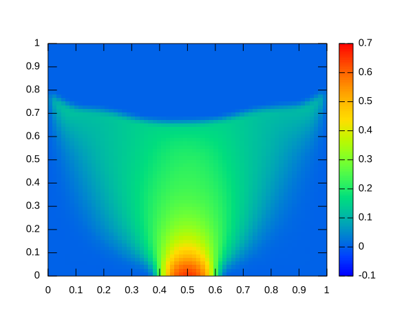
set terminal postscript color enhanced set output “t2vy.eps” replot
Plot of pressure at time 2
 reset
 set pm3d map
 set pm3d; set palette rgbformulae 22,13,-31;
 splot 'field-2.txt' u 1:2:(abs($4)**$3) with pm3d notitle
 set label "pressure" at graph 0.45, 0.85 font ",24" front
 set terminal postscript color enhanced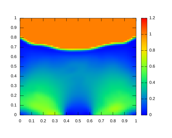
set output “t2p.eps” replot
Plot of viscosity at time 2
 reset
 set cbrange [0:2]
 set pm3d map
 set pm3d; set palette rgbformulae 22,13,-31;
 set label "Viscosity" at graph 0.45, 0.85 font ",24" front
 splot 'field-2.txt' u 1:2:(abs($14)**$3) with pm3d notitle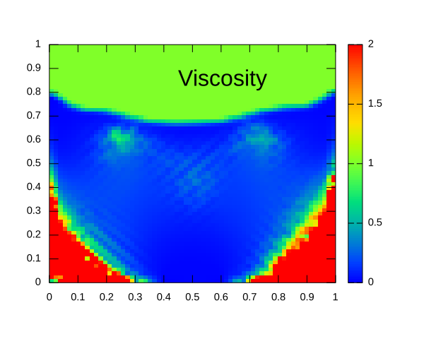
set terminal postscript color enhanced set output “t2eta.eps” replot
Links
https://basilisk.fr/sandbox/yixian/granular_bottom_NGF.c
https://basilisk.fr/sandbox/yixian/granular_bottom_constantNGF.c
https://basilisk.fr/sandbox/yixian/granular_bottom_dynamicNGF.c
https://basilisk.fr/sandbox/yixian/granular_bottom_linearisedconstantNGF.c
https://basilisk.fr/sandbox/yixian/granular_bottom_linearisedNGF.c
https://basilisk.fr/sandbox/yixian/granular_bottom_Local.c
https://basilisk.fr/sandbox/yixian/granular_bottom_muItheta.c
https://basilisk.fr/sandbox/yixian/granular_bottom_Igradient.c
Bibliography
Y. Zhou PhD https://theses.fr/2016AIXM4731
L. Staron, P.-Y. Lagrée, & S. Popinet (2014)
“Continuum simulation of the discharge of the granular silo, A validation test for the μ(I) visco-plastic flow law”
Eur. Phys. J. E (2014) 37: 5 DOI 10.1140/epje/i2014-14005-6L. Staron, P.-Y. Lagrée & S. Popinet (2012)
“The granular silo as a continuum plastic flow: the hour-glass vs the clepsydra”
Phys. Fluids 24, 103301 (2012); doi: 10.1063/1.4757390Kamrin, K. and Koval, G. (2012). Nonlocal constitutive relation for steady granular flow. Phys. Rev. Lett., 108:178301.