sandbox/walmetz/slip-length/navier_BC.c
This code was first written by Francesco Picella. I modified it a bit to use it my way.
//#include "grid/multigrid.h"
#include "grid/quadtree.h"
//#include "embed.h"
#include "twitkamp/MovingEmbed/embed_navier.h"
#include "navier-stokes/centered.h"
#include "view.h"

#define R0 0.5 // solid cylinder radius
#define xc 0.
#define yc 0.
#define T 25.

int MAXLEVEL = 10;
int MINLEVEL = 7;

face vector muv[];

// Fields that will contain the slip length...
scalar lambdax[], lambday[];

double slip;
double knudsen;

double Reynolds;

int main() {
  size (32.);
We set the origin
  origin (-8, -L0/2.); // at least 8 diameters beyond the inlet face
// so to avoid influence of confinement...
We enter parameters :
  double list_kn[] = {0.01, 0.03, 0.05, 0.08, 0.1, 0.3, 0.5, 0.8, 1.};
  double list_re[]= {20., 50., 100.}; //same Re as Legendre et al.,2009

  int size_kn = sizeof(list_kn) / sizeof(list_kn[0]);
  int size_re = sizeof(list_re) / sizeof(list_re[0]);
And we loop
  for (int i_re=0 ; i_re < size_re ; i_re++){

    Reynolds = list_re[i_re];

    for (int i_kn=0 ; i_kn < size_kn ; i_kn++){

      knudsen = list_kn[i_kn];
      slip = knudsen * R0; //Knudsen is easier to use, but embed_navier needs slip

      init_grid (1 << (MAXLEVEL-2)); //I'm not sure it has to be inside the loops but it works like this...

      mu = muv;

      run();
    }
  }
}
We set the boundary conditions, so to obtain a flow around a fixed cylinder.
u.n[left]  = dirichlet(1.0);
p[left]    = neumann(0.);
pf[left]   = neumann(0.);

u.n[right] = neumann(0.);
p[right]   = dirichlet(0.);
pf[right]  = dirichlet(0.);
Must impose no-slip on embedded boundaries!, even though we have a navier condition
u.n[embed] = dirichlet(0.);
u.t[embed] = dirichlet(0.);

event properties (i++)
{
  foreach_face()
    muv.x[] = fs.x[]*R0*2./Reynolds;
}

event init (t = 0)
{
We define the solid cylinder (EMBED) and fluid cylinder (PLASTRON) interface.
  solid (cs, fs, (sq(x - xc) + sq(y - yc) - sq(R0)));

// Initialize slip field as well for embed_navier.h
// The slip length is an scalar field attribute defined in embed_navier.h
  foreach(){
    lambdax[] = slip;
    lambday[] = slip;
  }
  u.x.lambda = lambdax;
  u.y.lambda = lambday;
// If the former values are not provided, the code will run...
// ...but providing non-sense values to slip lengths lambdas!
}

event adapt (i++) {
  adapt_wavelet ({cs,u}, (double[]){1e-3,1e-2,1e-2}, MAXLEVEL, MINLEVEL);
}
We finally compute forces and print them (with parameters first
event compute_forces (i++, t<=T)
{
  coord Fp, Fmu;
  embed_force (p, u, mu, &Fp, &Fmu);
    double Cx = (Fp.x+Fmu.x)*2.;
    double Cy = (Fp.y+Fmu.y)*2.;
    fprintf (stderr, "%+3.2e %+3.2e %06d %+6.5e %+6.5e %+6.5e %+6.5e %+6.5e %+6.5e %+6.5e %+6.5e\n",
             Reynolds, knudsen, i, t, dt, Cx, Cy, Fp.x, Fp.y, Fmu.x, Fmu.y);
    fflush (stderr);

}
If we need to visualise what we’re doing (it slows down the computing) :
//event movie(i+=100, t<=T){
//  view(fov=5, tx = 0, ty = 0);
//  draw_vof("cs", "fs",filled = -1);
  //draw_vof ("f", filled = 1, fc = {1,0,0});
 //draw_vof ("f", lc = {1, 0, 0}, lw = 2);
// squares ("u.x", linear = true);
 // Draw grid only on upper part of flow
// cells (lc = {0.7, 0.7, 0.7});
//
//
//  save("movie.mp4");
//}


//event movies (i += 10)
//{
//  scalar omega[], m[];
//  vorticity (u, omega);
//  foreach()
//    m[] = cs[] - 0.5;
//  output_ppm (omega, file = "vort.mp4", box = {{-0.5,-0.5},{7.5,0.5}},
//     min = -10, max = 10, linear = true, mask = m);
//}
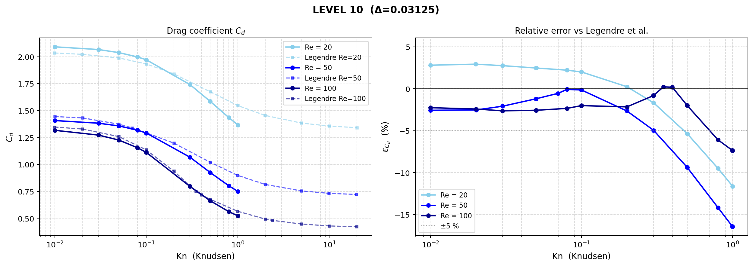
I’m not able to run the code on basilisk.fr, so there is no gnuplot link… I ran it using matplotlib and here are the results compared to Legendre et al.,2009
It appears we’re near their results for Kn < 0.1, for each reynolds (and each LEVEL superior to 9). Physically, it shouldn’t exceed 0.1, so we can validate the code with an accuracy of within 5% compared to Legendre.