2D_cylinder.c

Code by F.Picella (original) modified to suppress multiphase flow and model a simple 2D cylinder.

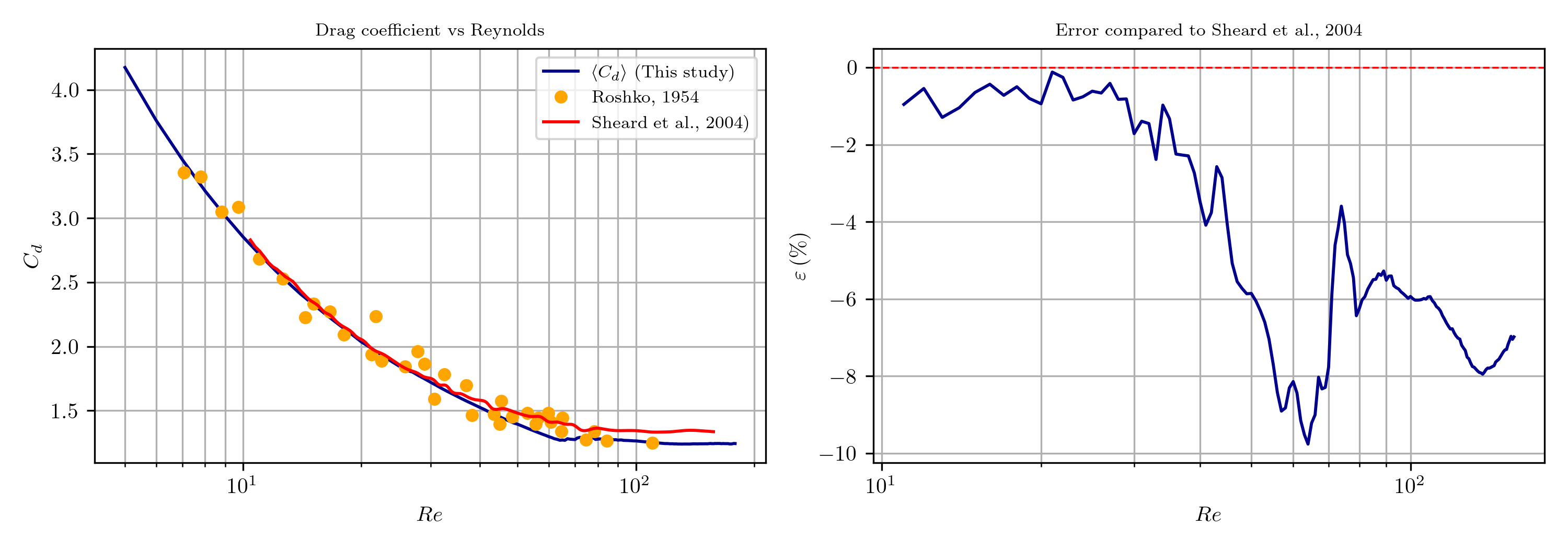
I just want to validate it by comparing it to a typical (Cd,Re) diagram (Roshko,1960).

//#include "grid/multigrid.h"
#include "embed.h"
#include "navier-stokes/centered.h"
#include "two-phase.h"
//#include "tension.h"
//#include "tavares/contact-embed.h"
#include "view.h"

#define R0 0.5 // solid cylinder radius
#define xc 0.
#define yc 0. 
#define T 100.

int LEVEL = 10;

double Reynolds;

int main() {
  size (32.);

We set the origin

  origin (-8, -L0/2.);

  // boucle sur les LEVEL
  for ( Reynolds = 5 ; Reynolds < 180 ; Reynolds++){


    init_grid (1 << LEVEL);

We use a constant viscosity.

        mu2 = 1.*R0*2./Reynolds; // outer fluid viscosity 

        run();
   }
}

We set the boundary conditions, so to obtain a flow around a fixed cylinder.

u.n[left]  = dirichlet(1.0);
p[left]    = neumann(0.);
pf[left]   = neumann(0.);

u.n[right] = neumann(0.);
p[right]   = dirichlet(0.);
pf[right]  = dirichlet(0.);

Must impose no-slip on embedded boundaries!

u.n[embed] = dirichlet(0.);
u.t[embed] = dirichlet(0.);

event init (t = 0)
{

We define the solid cylinder (EMBED) and fluid cylinder (PLASTRON) interface.

  solid (cs, fs, (sq(x - xc) + sq(y - yc) - sq(R0)));

}

event adapt (i++) {
  adapt_wavelet ({cs,u}, (double[]){1e-2,3e-2,3e-2}, LEVEL, LEVEL-3);
}

event compute_forces (i++, t<=T)
{
  coord Fp, Fmu;
  embed_force (p, u, mu, &Fp, &Fmu);
    double Cx = (Fp.x+Fmu.x)*2.;
    double Cy = (Fp.y+Fmu.y)*2.;
    fprintf (stderr, "%+3.2e %06d %+6.5e %+6.5e %+6.5e %+6.5e \n",
             Reynolds, i, t, dt, Cx, Cy);
    fflush (stderr);
}

If we need to visualise what we’re doing (it slows down the computing) :

//
//event movie(i+=10,t<=T){
//  view(fov=5, tx = 0, ty = 0);
//  draw_vof("cs", "fs",filled = -1);
  //draw_vof ("f", filled = 1, fc = {1,0,0});
//        draw_vof ("f", lc = {1, 0, 0}, lw = 2);
//        squares ("u.x", linear = true);
        // Draw grid only on upper part of flow
//        cells (lc = {0.7, 0.7, 0.7});


//  save("movie.mp4");
//}

Finally, we plot the drag coefficient C_d as a function of the Reynolds number Re, and we compare our results with the experimental data of Roshko, 1954 (taken on Persillon et Braza, 1998), and the numerical results of Sheard et al., 2005. On the left panel, the first one is represented by the orange circles, while the second one is shown as the red curve. On the right panel, we use the numerical study to compute the error \varepsilon.

Although this cylinder case has been studied for more than a century, no universally accepted reference curve exists. Therefore, even though there is a near 10% error for some Re, we will consider our code to be valid.

The plots are shown for Reynolds numbers between 5 and 180 (with a step of 1), since the wake instability becomes three-dimensional above Re≈180.

Results compared to other studies