porous-plug.c

Porous plug flow with Darcy’s law

Porous plug flow with Darcy’s law

This case simulates a laminar flow through a porous plug using Darcy’s law to account for the resistance induced by the porous media. The plug is placed in the middle of the domain. The flow is driven by a constant inlet velocity on the left boundary and a zero pressure condition on the right boundary. The velocity profile and pressure drop across the plug are compared with the analytical solution.

#define POROUS_ADVECTION 1
#define NO_DARCY_CORRECTION 1
#include "navier-stokes/centered-phasechange.h"
#include "fractions.h"
#include "darcy.h"

Simulation parameters

double U0 = 0.8;      // inlet velocity
int maxlevel = 10;    // maximum refinement level
double eps0 = 0.6;    // porosity of the plug
double rhoG = 1.;     // density of the fluid
double muG = 1e-1;    // viscosity of the fluid
double K = 1e-4;      // permeability of the plug

Boundary conditions

Uniform inlet velocity profile on the left boundary and zero pressure on the right boundary. Symmetry conditions on top and bottom boundaries.

u.n[left] = dirichlet (U0);
u.t[left] = dirichlet (0.);
p[left] = neumann (0.);
pf[left] = neumann (0.);

u.n[right] = neumann (0.);
u.t[right] = neumann (0.);
p[right] = dirichlet (0.);
pf[right] = dirichlet (0.);

Main function

We set the fluid properties, domain size and permeability of the plug.

face vector muv[];

int main () {
  const face vector muv[] = {muG, muG};
  mu = muv;

  const scalar rhov[] = rhoG;
  rho = rhov;

  Da = (coord) {K, K};
  init_grid (1 << maxlevel);
  run();
}

Initialization

We define the porous plug in the middle of the domain, between x=0.4 and x=0.6.

scalar porosity[], f[];
event init (i = 0) {
  fraction (f, (x - 0.4)*(0.6 - x));

  scalar eps[];
  foreach() {
    porosity[] = f[]*eps0;
    eps[] = eps0*f[] + (1. - f[]);
    u.x[] = U0;
  }

  scalar centered_mu[];
  foreach()
    centered_mu[] = muG/eps[];

  foreach_face()
    muv.x[] = face_value(centered_mu, 0);
}

CFL condition

We limit the maximum CFL number to ensure stability. Also consider that, when looking at the steadystate solution using an operator splitting method, the solution value is sensitive to the timestep. See Septh et al. 2013 for more details.

const double max_cfl = 0.1;
event stability (i++) {
  if (CFL > max_cfl)
    CFL = max_cfl;
}

Log and stop event

After few iterations, the solution reaches a steady state. We log the velocity and pressure profiles for comparison with the analytical solution.

event logprofile (t = end) {
  for (double x = 0.; x < L0; x += L0/(1<<maxlevel))
    fprintf (stderr, "%g %g %g\n", x, 
                                   interpolate (u.x, x, 0.5), 
                                   interpolate (p, x, 0.5));
}

event stop (i  = 10);

Post-processing

reset
set terminal svg size 700, 350  
set output "plot.svg"

set multiplot layout 1,2

set xlabel "x"
set ylabel "Velocity"
set yrange [0:2]
unset key
set samples 20
set size square
set xtics 0.2

set object 1 rectangle from 0.4,graph 0 to 0.6,graph 1 behind fc "black" fs solid 0.2

u_in = 0.8
analytical_u(x) = u_in

plot "log" u 1:2 w l lc "black" t "u", \
     analytical_u(x) w p pt 4

set xlabel "x"
set ylabel "Pressure"
set samples 20
unset key
set size square
set yrange [-10:250]
set xtics 0.2

set object 1 rectangle from 0.4,graph 0 to 0.6,graph 1 behind fc "black" fs solid 0.2

mu = 1e-1
u_in = 0.8
epsilon = 0.6
K = 1e-4
rho = 1
F = 1.75/sqrt (150*epsilon**3)
B = mu*u_in/K + rho*F*epsilon*u_in*u_in/K**0.5
analytical_p(x) = (x < 0.4) ? B*(0.6-0.4) : \
                  (x > 0.6) ? 0 : \
                  rho*u_in*u_in*(1-1/epsilon) + B*(0.4-x + (0.6-0.4))

plot "log" u 1:3 w l lc "black" t "p", \
     analytical_p(x) w p pt 4

unset multiplot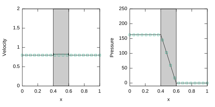

References

[speth2013balanced]

Raymond L Speth, William H Green, Shev MacNamara, and Gilbert Strang. Balanced splitting and rebalanced splitting. SIAM Journal on Numerical Analysis, 51(6):3084–3105, 2013.