porous-channel.c

Porous channel flow

Porous channel flow

This case simulates the flow in a 2D channel partially filled with a porous medium. The porous medium occupies the lower half of the channel, while the upper half is free fluid. Velocity at the inlet is uniform and let to develop along the channel length. The simulation parameters are chosen to match the results reported by Betchen et al. (2006).

Simulation parameters

Particular attention must be given to the U0 value at the inlet. As the original paper, we have to set U0 so that Re number is 1 in the free fluid region when the profile is fully developed. This turns out to be U \approx 1 or U0 = 1.17 for the current case. This is verified by computing the average velocity in the free fluid region at the outlet, as done in the stop event.

“POROUS_ADVECTION” overloads some steps of the Navier-Stokes solver to account for a porous medium. In this case this effect is minimal and using centered.h work fine aswell.

#define POROUS_ADVECTION 1

int maxlevel = 9;        // Maximum refinement level
double H = 1.;            // Channel height
double U0 = 1.17;       // Inflow velocity for Da = 1e-2
//double U0 = 1.05;       // Inflow velocity for Da = 1e-3
double eps0 = 0.7;        // Porosity
double tend = 10.;         // End time
double Re = 1.;           // Reynolds number

scalar eps[];

#include "grid/multigrid.h"
#include "navier-stokes/centered-phasechange.h"
#include "fractions.h"
#include "darcy.h"
#include "view.h"

Boundary conditions

left: inlet only in the free fluid region
right: outlet
top: wall
bottom: wall

u.n[left] = dirichlet (U0*(1. - f[]));
u.t[left] = dirichlet (0.);
p[left] = neumann (0.);
pf[left] = neumann (0.);

u.n[right] = neumann (0.);
u.t[right] = neumann (0.);
p[right] = dirichlet (0.);
pf[right] = dirichlet (0.);

u.n[top] = dirichlet (0.);
u.t[top] = dirichlet (0.);
p[top] = neumann (0.);
pf[top] = neumann (0.);

u.n[bottom] = dirichlet (0.);
u.t[bottom] = dirichlet (0.);
p[bottom] = neumann (0.);
pf[bottom] = neumann (0.);

scalar porosity[], f[];
double rhoG = 1., muG;
face vector muv[];

int main() {

We download data for post-processing.

  system ("wget https://raw.githubusercontent.com/Riccaraccio/basilisk-sandbox-rcaraccio/refs/heads/master/data/porouschannel/velocity-da-02");

We set the fluid properties to match the desired Re number in the free fluid region.

  muG = H*1.*rhoG/Re;
  mu = muv;

  Da = (coord) {1.e-2*sq(H), 1.e-2*sq(H)};

The domain is 8H x 2H

  size (8*H);
  dimensions (nx=8, ny=2);
  
  origin (0, -H);
  init_grid (1 << maxlevel);

  run();
}

We initialize the porous medium in the lower half of the channel.

event init (i = 0) {
  fraction (f, -y);
  foreach() {
    porosity[] = f[]*eps0;
    eps[] = eps0*f[] + (1. - f[]);
  }

In the porous region, the fluid is more viscous due to the presence of the solid matrix.

  scalar centered_mu[];
  foreach()
    centered_mu[] = muG/eps[];

  foreach_face()
    muv.x[] = face_value(centered_mu, 0);
}

We restrict the maximum CFL number to 0.1 to ensure stability.

const double cfl_max = 0.1;
event stability (i++) {
  if (CFL > cfl_max)
    CFL = cfl_max;
}

Log event

We log the velocity profile at near the outflow region. We also compute the average velocity in the free fluid region, it should be close to 1.

void write_results() {
  double step = 2*H/(1 << maxlevel);
  double x_interpolate = 0.999*8*H;
  int counter = 0;

  // Compute average velocity in free fluid region
  double avg_U = 0.;
  for (double y = 0; y<H; y+=step){
    double U = interpolate (u.x, x_interpolate, y);
    counter++;
    avg_U += U;
  }
  avg_U /= counter;

  for (double y = -H; y<H; y+=step){
    double Y = y/H;
    double U = interpolate (u.x, x_interpolate, y);
    fprintf (stderr, "%g %g\n", U/avg_U, Y);
  }
  fprintf (stderr, "# Avg u: %g\n", avg_U);
}

We stop the simulation after convergence of the flow filed is reached

scalar un[];
#define CONVERGENCE_TOLERANCE 1e-10

event steadystate (i++) {
  double du = change (u.x, un);
  if (i > 1 && du < CONVERGENCE_TOLERANCE) {
    fprintf (stderr, "# Steady state reached after %d iterations %g time \n", i, t);
    write_results();
    return 1;
  }
}

event stop (t = tend) {
  write_results();
}

Velocity profile plot

reset
set terminal svg size 400,400
#set terminal epslatex color size 3.6, 3.6
set output "porous-channel-da-02.svg"

set xlabel "u/U"
set ylabel "y/H"
set grid
set xtics 0.25
set size square
unset key

set xrange [0:1.5]
set yrange [-1:1]
plot  "log" u 1:2 w l lw 3 lc "black" t "Simulation", \
      "velocity-da-02" w p pt 64 ps 1.2 lw 3 lc "black" t "Betchen et al. (2006)"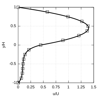

References

[betchen2006]

Lee Betchen, Anthony G Straatman, and Brian E Thompson. A nonequilibrium finite-volume model for conjugate fluid/porous/solid domains. Numerical Heat Transfer, Part A: Applications, 49(6):543–565, 2006.