sandbox/jmerrifield/Sessile/sessile_embed_grav.c
Sessile drop subject to gravity on an embedded boundary
e_th = 1.24e-02
e_inf(Bo) = 2.0*0.01*sin(130*pi/180./2.0)/sqrt(Bo)/e_th

set key bottom left

set logscale x
set yrange [0:1.5]
set xlabel "Bond number Bo"
set ylabel "Dimensionless width e*"
set grid

plot "e_theta_130.dat" u 1:2 w lp title "Numerical", \
        1. w l lc rgb "black" dt 2 title "Theoretical geometric thickness", \
        [1e-3:1e2] e_inf(x) w l lc rgb "black" dt 3 title "Thickness due to gravity"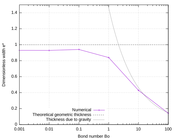
// fixme :  voir pourquoi la récupération des données pour le graphe en fonction
// de Bo ne fonctionne pas et donne des données différentes dans fp4 que dans fp2


#include "twitkamp/MovingEmbed/embed_navier.h"
#include "navier-stokes/centered.h"
#include "two-phase.h"
#include "tension.h"
#include "tavares/contact-embed.h"
#include "view.h"
#include "jmerrifield/interface_properties.h"

//Dimensionless numbers
double Bo;
double Oh;

double ywall;

//Physical parameters
double rho1, rho2, mu1, mu2;

//Geometrical parameters
double R0 = 0.01;
double h = 0.006;
double xc, yc;

double r_th, e_th, l_th;
double e;
double rf, hf;
double r;

double theta0 = 130.; // Contact angle in degrees

double V0 = 0., Vf = 0.;

//Slip length
double slip = 0.;
scalar lambdax[], lambday[];


// // Domain parameters
int level = 7;

double domainSize = 12; // relative domain size wrt R

double endTime = 2.;

SessileData last_contact;

face vector muv[];
face vector av[];

FILE *fp1;
FILE *fp2;
FILE *fp3;
FILE *fp4;
FILE *fp5;
FILE *fp6;

int main()
{
  //Domain definition
  L0 = domainSize*R0;
  N = 1 << level;   // <=> N = 2^{minlevel}
  origin (-L0/2.,-L0/2.);

  //Physical parameters
  rho1 = 1000.;
  rho2 = 1.;
  mu1 = 0.01;
  mu2 = 1e-5;

  f.sigma = 0.072;
  a = av;
  mu = muv;

  char filename4[100];
  sprintf(filename4, "e_theta_%g.dat", theta0);
  fp4 = fopen(filename4, "w");
  fprintf(fp4, "Bo e \n");
Contact angle
We impose a constant contact angle at the embed boundary.
  const scalar c[] = theta0*pi/180.;
  contact_angle = c;
/*
The Bond number is varied to vary the influence of the gravity.
*/
  for (Bo=0.001; Bo<=100; Bo*=10)
  {
    fprintf(stderr,"\n===== Simulation Bo %g =====\n", Bo);
    run();
  }
}
Boundary conditions
We set the boundary conditions for a sessile that can slip partially at the embed boundary.
//Lower conditions
u.t[bottom] = dirichlet(0.);

//Upper conditions
u.t[top]   = dirichlet(0.);

//Right conditions
u.t[right] = dirichlet(0.);

//Left conditions
u.t[left] = dirichlet(0.);

//Non-slip and non-penetration conditions on the walls
u.n[embed] = dirichlet(0.);
u.t[embed] = dirichlet(0.);

//Initial conditions
event init (t = 0)
{
  ywall = -L0/2. + h;

  // Definition of solid walls
  solid (cs, fs,
         y - ywall);

  // Initial position of the liquid
  xc = L0/(2.*N);
  yc = ywall - L0/(2.*N);
  fraction (f,
            min(sq(R0) - sq(x - xc) - sq(y - yc),
                y-yc));
Navier slip
We set here the slip length used for the partial slip.
  foreach()
  {
    lambdax[] = L0/(2.*N);
    lambday[] = 0.;
  }
  u.x.lambda = lambdax;
  u.y.lambda = lambday;

  //Volume conservation
  foreach(reduction(+:V0))
    V0 += f[]*cs[]*dv();
}

event file (t=0)
{
  //File opening
  char filename[100];
  sprintf(filename, "properties_theta_%g_Bo_%g.dat", theta0, Bo);
  fp1 = fopen(filename, "w");

  char filename2[100];
  sprintf(filename2, "Ca_theta_%g_Bo_%g.dat", theta0, Bo);
  fp2 = fopen(filename2, "w");

  char filename3[100];
  sprintf(filename3, "data_Bo_%g.dat", Bo);
  fp3 = fopen(filename3, "w");

  char filename5[100];
  sprintf(filename5, "facets_Bo_%g.dat", Bo);
  fp5 = fopen(filename5, "w");

  fp6 = fopen("solids.dat", "w");

  //File definition
  fprintf(fp1, "t x_g x_d r U_g U_d theta_g theta_d e \n");
  fprintf(fp2, "t Ca_g Ca_d \n");

  Oh = (mu1)/sqrt(rho1*f.sigma*R0);
  fprintf(fp3, "Oh = %3.2e \n", Oh);
  double t = theta0*pi/180.;
  r_th = R0*sqrt(pi/(2*(t - sin(t)*cos(t))));
  fprintf(fp3, "R_th = %3.2e \n", r_th);
  l_th = 2*r_th*sin(t);
  fprintf(fp3, "L_th = %3.2e \n", l_th);
  e_th = r_th*(1 - cos(t));
  fprintf(fp3, "e_th = %3.2e \n", e_th);

  fprintf(fp3, "V0 = %g \n", V0);
}
Gravity
The gravity is set to vary with the Bond number to see its influence on teh sessile shape.
event acceleration (i++, t<=endTime)
{
  foreach_face(y)
    av.y[] -= Bo*f.sigma/(rho1*sq(R0));
}

event logfile (t+=0.05)
{
  SessileData c = contact_properties(f, cs, fs, ywall);

  r = (c.x_right - c.x_left)/2.;

  fprintf(fp1,
          "%6.5e %6.5e %6.5e %6.5e %6.5e %6.5e %6.5e %6.5e %6.5e \n",
          t,
          c.x_left - L0/(2.*N),
          c.x_right - L0/(2.*N),
          r,
          c.U_left,
          c.U_right,
          c.theta_left,
          c.theta_right,
          c.height
         );

  fprintf(fp2, "%6.5e %6.5e %6.5e \n", t, mu1*c.U_left/f.sigma, mu1*c.U_right/f.sigma);

  last_contact = contact_properties(f, cs, fs, ywall);
}

// Actions at the end of the simulation
event end (t = end)
{
  //Interface recuperation
  output_facets (f, fp5);
  output_facets (cs, fp6);
  // Volume conservation
  foreach(reduction(+:Vf))
    Vf += f[]*cs[]*dv();
  fprintf(fp3, "Vf = %g \n", Vf);

  // Height VS Bo
  SessileData c = contact_properties(f, cs, fs, ywall);
  fprintf(fp4, "%6.5e %6.5e \n ", Bo, c.height/e_th);
  fclose (fp1);
}
References
| [legendre_comparison_2015] |
D. Legendre and M. Maglio. Comparison between numerical models for the simulation of moving contact lines. Computers & Fluids, 113:2–13, May 2015. [ DOI | http ] |
//fixme : see why the file fp4 is empty for the graph