sandbox/jmerrifield/Sessile/sessile_embed.c
Sessile drop on an embedded boundary
In this code, I wanted to compare different contact angle models : simplified Cox-Voinov and Afkhami model for dynamic contact angle models and static contact angle model
Cox-Voinov Law
Cox gives a formula for dynamic contact that simplifies to the formula below if \theta_d < 3 \pi /4 : \theta_d^3 = \theta_S^3 + 9Ca\ln\left(\frac{L}{\lambda}\right)
Afkhami model
Afkhami proposed a model based for 2D simulations and Cox expression that reduced to : \cos\theta_d = \cos\theta_S + 5.63 Ca \ln\left(\frac{K}{\Delta/2}\right)
r_th = 1.38/2.

Ndyn = 4
Nstat = 3
Ntot = Ndyn + Nstat

set key bottom right

set xlabel "Time (s)"
set ylabel "Half width (m)"
set grid

plot \
for [i=1:Ndyn] \
        sprintf("properties_Dyn%d.dat", i) \
            u 1:4 w lp lw 2 title sprintf("Dyn %d", i), \
for [j=1:Nstat] \
            sprintf("properties_Stat%d.dat", j) \
            u 1:4 w lp lw 2 title sprintf("Stat %d", j), \
        r_th w l lc rgb "black" dt 2 title "Theoretical half width"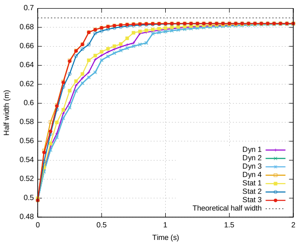
#include "twitkamp/MovingEmbed/embed_navier.h"
#include "navier-stokes/centered.h"
#include "two-phase.h"
#include "tension.h"
#include "tavares/contact-embed.h"
#include "view.h"
#include "jmerrifield/interface_properties.h"

typedef struct {
  char *name;
  int contact_model;
  double L;
  int slip_model;
} Case;

#define STATIC    0
#define COXVOINOV 1
#define AFKHAMI   2

#define SLIP_NONE    0
#define SLIP_HALF    1
#define SLIP_32_HALF 2
Definition of the test cases
The different test cases are listed below.
| Model name | Contact angle | Navier condition |
|---|---|---|
| Stat1 | \theta_w=\theta_S | \lambda_N=0 |
| Stat2 | \theta_w=\theta_S | \lambda_N=\Delta/2 |
| Stat3 | \theta_w=\theta_S | \lambda_N=\Delta_{32}/2 |
| Dyn1 | \theta_w=\theta_d (Eq. Simplified Cox-Voinov) with L=10^{-6}, \lambda=10^{-9}\,\mathrm{m} | \lambda_N=0 |
| Dyn2 | \theta_w=\theta_d (Eq. Simplified Cox-Voinov) with L=\Delta/2, \lambda=10^{-9}\,\mathrm{m} | \lambda_N=0 |
| Dyn3 | \theta_w=\theta_d (Eq. Simplified Cox-Voinov) with L=\Delta/2, \lambda=10^{-9}\,\mathrm{m} | \lambda_N=\Delta/2 |
| Dyn4 | \theta_w=\theta_d (Eq. Afkhami 2009) | \lambda_N=\Delta/2 |
Case cases[7] = {

  {"Stat1", STATIC,    0.,        SLIP_NONE},
  {"Stat2", STATIC,    0.,        SLIP_HALF},
  {"Stat3", STATIC,    0.,        SLIP_32_HALF},

  {"Dyn1",  COXVOINOV, 1e-6,      SLIP_NONE},
  {"Dyn2",  COXVOINOV, 0.,        SLIP_NONE},
  {"Dyn3",  COXVOINOV, 0.,        SLIP_NONE},

  {"Dyn4",  AFKHAMI,   0.,        SLIP_HALF}
};

//Dimensionless numbers
double Ca_g, Ca_d;
double Oh;
//double La;
//double We;

//Boundary velocity
double ux_wall;
double uy_wall;
double xCL;
double yCL;
double ywall;

//Physical parameters
double rho1, rho2, mu1, mu2;

//Geometrical parameters
double R0 = 0.5;
double h = 0.26;
double xc, yc;

double r_th, e_th, l_th;
double rf, hf;
double r;

double theta0 = 60.; // Contact angle in degrees

double V0;

//Slip length
double slip;
scalar lambdax[], lambday[];

int level = 6;

double endTime = 2.;

face vector muv[];
face vector av[];

FILE *fp1;
FILE *fp3;

//Simulation parameters
int contact_model;
double L;
int slip_model;
int icase;
Case cas;

int main()
{
  //Domain definition
  L0 = 2.;
  N = 1 << level;
  origin (-L0/2.,-L0/2.);

  //Physical parameters
  rho1 = 1.;
  rho2 = 1.;
  mu1 = 0.25;
  mu2 = 0.25;

  f.sigma = 7.5;
  a = av;
  mu = muv;

  for (icase = 0; icase < 7; icase++)
  {

    cas = cases[icase];

    fprintf(stderr, "Running %s\n", cas.name);

    if (cas.contact_model == COXVOINOV && cas.L == 0.)
    {
      cas.L = L0/N/2.;
    }
    contact_model = cas.contact_model;

    switch (cas.slip_model)
    {
      case SLIP_NONE:
        slip = 0.;
        break;

      case SLIP_HALF:
        slip = L0/N/2.;
        break;

      case SLIP_32_HALF:
        slip = L0/32/2.;
        break;
    }

    run();
  }
}
Boundary conditions
We set the boundary conditions for a sessile that can slip partially at the embed boundary.
//Lower conditions
u.t[bottom] = dirichlet(0.);

//Upper conditions
u.t[top]   = dirichlet(0.);

//Right conditions
u.t[right] = dirichlet(0.);

//Left conditions
u.t[left] = dirichlet(0.);

//Navier slip and non-penetration conditions on the plane
u.n[embed] = dirichlet(0.);
u.t[embed] = dirichlet(0.);

//Initial conditions
event init (t = 0)
{
  ywall = -L0/2. + h;

  // Definition of solid walls
  solid (cs, fs,
         y - ywall);

  // Initial position of the liquid
  xc = L0/(2.*N);
  yc = ywall - L0/(2.*N);
  fraction (f,
            min(sq(R0) - sq(x - xc) - sq(y - yc),
            y-yc));
Navier slip
We set here the slip length used for the partial slip.
  foreach()
  {
    lambdax[] = slip;
    lambday[] = 0.;
  }
  u.x.lambda = lambdax;
  u.y.lambda = lambday;
}

// File opening
event file (t=0)
{
  //File opening
  char filename[100];
  sprintf(filename, "properties_%s.dat", cas.name);
  fp1 = fopen(filename, "w");

  fp3 = fopen("data.dat", "w");

  //File definition
  fprintf(fp1, "t x_g x_d r U_g U_d theta_g theta_d e \n");

  Oh = (mu1)/sqrt(rho1*f.sigma*R0);
  fprintf(fp3, "Oh = %3.2e \n", Oh);
  double t = theta0*pi/180.;
  r_th = R0*sqrt(pi/(2*(t - sin(t)*cos(t))));
  fprintf(fp3, "R_th = %3.2e \n", r_th);
  l_th = 2*r_th*sin(t);
  fprintf(fp3, "L_th = %3.2e \n", l_th);
  e_th = r_th*(1 - cos(t));
  fprintf(fp3, "e_th = %3.2e \n", e_th);
}
Dynamic contact angle
We compute the contact angle at the embed boundary with multiple contact angle models (static and dynamic).
event switch_angle (i++, t<=endTime)
{
  if (contact_model == STATIC)
  {
    const scalar theta[] = theta0*pi/180.;
    contact_angle = theta;
  }

  else
  {
    SessileData c = contact_properties(f, cs, fs, ywall);
    double Ca = fabs(mu1*c.U_right/f.sigma);

    if (contact_model == COXVOINOV)
    {
      double lambda = 1e-9;
      double a = pow((theta0*pi/180.),3) + fabs(Ca)*log(cas.L/lambda);
      double theta_dyn = pow(a, 1./3.);
      const scalar theta[] = theta_dyn;
      contact_angle = theta;
    }

    if (contact_model == AFKHAMI)
    {
      double K = 0.04*R0;
      double a = cos(theta0*pi/180.) + 5.63*fabs(Ca)*log(K/(L0/(2.*N)));
      double b = max(-1., min(1.,a));
      double theta_dyn = acos(b);
      const scalar theta[] = theta_dyn;
      contact_angle = theta;
    }
  }
}

event logfile (t+=0.05)
{
  SessileData c = contact_properties(f, cs, fs, ywall);

  r = (c.x_right - c.x_left)/2.;

  fprintf(fp1,
          "%6.5e %6.5e %6.5e %6.5e %6.5e %6.5e %6.5e %6.5e %6.5e \n",
          t,
          c.x_left - xc,
          c.x_right - xc,
          r,
          c.U_left,
          c.U_right,
          c.theta_left,
          c.theta_right,
          c.height
         );
}

event end (t = end)
{
  fclose (fp1);
  fclose (fp3);
}
References
| [legendre_comparison_2015] |
D. Legendre and M. Maglio. Comparison between numerical models for the simulation of moving contact lines. Computers & Fluids, 113:2–13, May 2015. [ DOI | http ] |