sandbox/jmerrifield/Capillary/capillary_embed_noslip.c
Capillary with no slip boundary condition
set grid
set key bottom right
set yrange [:20.2]
set xlabel "Time (s)"
set ylabel "Height (mm)"
plot for [i=5:8] sprintf("h_interface_maxlevel_%d.dat",i) us 1:2 w lp \
        title sprintf("nx = %d, dx = %.2e",2**i,2*0.005/2**i), \
        19.9933 w l lc rgb "black" dt 2 title "2D Jurin's height", \
        19.1538 w l lc rgb "black" title "Corrected 2D Jurin's height"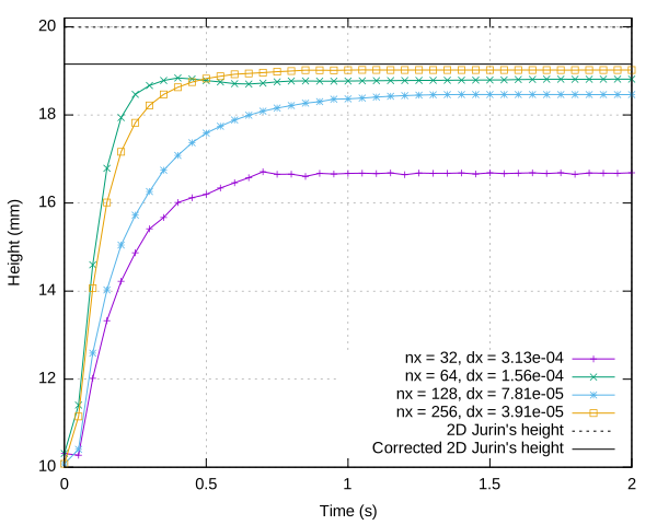
#include "embed.h"
#include "navier-stokes/centered.h"
#include "two-phase.h"
#include "tension.h"
#include "tavares/contact-embed.h"
#include "view.h"
#include "jmerrifield/interface_properties.h"

// Dimensionless numbers
double Bo;
double Oh;
double omega;

// Physical parameters
double rho1, rho2, mu1, mu2;
double grav = 4.17;
double tens = 0.04;

// Geometrical parameters
double e;
double R = 0.005;
double dx, dy;
double h_jurin;
double h_corr;
double h_wash;

double V0;
double theta0 = 30.;   // Contact angle in degrees
double beta = 0.;

// Domain parameters
int minlevel = 4;
int maxlevel;
double domainSize = 6.; // relative domain size wrt R

double endTime = 2.;

face vector muv[];
face vector av[];


FILE *fp1;
FILE *fp2;
FILE *fp3;
FILE *fp4;
FILE *fp5;
FILE *fp6;
FILE *fp7;
FILE *fp8;

int main() {
  // Domain definition
  L0 = domainSize*R;
  N = 1 << minlevel;
  origin (0.,0.);

  dx = R/N;
  dy = L0/N;
  //Wall thickness
  e = L0/2. - R;

  //Physical parameters
  rho1 = 83.1;
  rho2 = rho1/1000.;
  mu1 = 0.01;
  mu2 = mu1/1000.;
  f.sigma = tens;
  a = av;
  mu = muv;
Contact angle
We impose a constant contact angle at the embed boundary.
  const scalar theta[] = theta0*pi/180.;
  contact_angle = theta;
  for (maxlevel = 5; maxlevel <= 8; maxlevel++)
  {
    run();
  }
}
Boundary conditions
We set the boundary conditions for a capillary tube with each end opened (at the top and the bottom) so that the fluid can pass through this numerical boundary. In this test case, the fluid cannot slip at the embed boundary.
//Lower conditions
u.n[bottom]  = neumann(0.);
p[bottom] = dirichlet(0.);

//Upper conditions
u.n[top] = neumann(0.);
p[top] = dirichlet(0.);

//Non-slip and non-penetration conditions on the walls
u.n[embed] = dirichlet(0.);
u.t[embed] = dirichlet(0.);

event init (t = 0)
{
The interior of the canal is refined since it’s the zone of th domain where the fluid is. The refined zone is slightly lager than the canal.
  double R_factor = 1.5;
  refine (x > L0/2 - R*R_factor && x < L0/2 + R*R_factor && level < maxlevel);
  solid (cs, fs, min(x - e, (L0 - e) - x));

  fraction (f, y < 2*R && x > L0/2 - R && x < L0/2 + R);

  //Volume conservation
  //foreach(reduction(+:V0))
  //	V0 += f[]*cs[]*dv();
}

event file (t=0)
{
  //File opening
  fp1 = fopen("vitesses_max.dat", "w");

  char filename[100];
  sprintf(filename, "angle_maxlevel_%d.dat", maxlevel);
  fp2 = fopen(filename, "w");

  char filename2[100];
  sprintf(filename2, "h_interface_maxlevel_%d.dat", maxlevel);
  fp3 = fopen(filename2, "w");

  fp4 = fopen("data.dat","w");
  fp5 = fopen("Washburn.dat","w");

  fprintf(fp1, "t  u.x  u.y \n");
  fprintf(fp2, "t  theta \n");
  fprintf(fp3, "t  h \n");
}

event data_recuperation (t=0)
{
  //Canal length
  fprintf(fp4, "L = %g mm \n", 1000*L0);
  //Canal radius
  fprintf(fp4, "R = %g mm \n", 1000*R);
  //Spatial steps
  fprintf(fp4, "dx = %g mm \n", 1000*dx);
  fprintf(fp4, "dy = %g mm \n", 1000*dy);
  //Initial volume
  //fprintf(fp4, "V0 = %g mm³\n", pow(1000,3)*V0);

  //Bond number
  Bo = (rho1*pow(R,2)*grav)/f.sigma;
  fprintf(fp4, "Bo = %g \n", Bo);
  //Ohnesorge number
  Oh = mu1/(sqrt(rho1*f.sigma*R));
  fprintf(fp4, "Oh = %g \n", Oh);
  //Omega from Bosanquet equation
  omega = sqrt((9*f.sigma*cos(theta0*pi/180.)*pow(mu1,2))/(pow(rho1,3)*pow(grav,2)*pow(R,5)));
  fprintf(fp4, "omega = %g \n", omega);

  //2D Jurin height
  h_jurin = f.sigma*cos(theta0*pi/180.)/(rho1*grav*R);
  fprintf(fp4, "h_jurin = %g mm \n", 1000*h_jurin);
  //Corrected height
  h_corr = h_jurin - R/(2*cos(theta0*pi/180.))*(2 - sin(theta0*pi/180.) - asin(cos(theta0*pi/180.))/cos(theta0*pi/180.));
  fprintf(fp4, "h_corr = %g mm \n", 1000*h_corr);
}
Gravity
The gravity is set to be constant.
event acceleration (i++, t<=endTime)
{
  foreach_face(y)
    av.y[] -= grav;
}

event logfile (t+=0.05)
{
  //Velocity data
  stats V = statsf(u.y);
  stats U = statsf(u.x);
  fprintf(fp1, "%+6.5e %+6.5e %+6.5e\n", t, U.max, V.max);
}

// Meniscus height
event meniscus_height (t+=0.05)
{
  //Interface data
  CapData data = cap_properties (f, cs, beta, R);

  fprintf(fp2, "%+6.5e %+6.5e \n", t, data.theta_right);
  fprintf(fp3, "%+6.5e %+6.5e \n", t, 1000*data.h_int);
  //fprintf(fp6, "%+6.5e %+6.5e %+6.5e \n", t, pow(1000,3)*V, (data.V - V0)/V0);

  //Washburn height
  h_wash = sqrt(pow(2.*R,2) + (tens*R*cos(theta0*pi/180.))/(2.*mu1)*t);
  fprintf(fp5, "%+6.5e %+6.5e %+6.5e \n", t, 1000*data.h_int, 1000*h_wash);
}
Transient/dynamic state
The dynamic of evolution of the phenomenon is compared to the Lucas-Washburn law : \displaystyle h(t)=\sqrt{h_0^2 + \left[{\frac {R\cos \theta }{2}}\right]\left[{\frac {\sigma }{\mu }}\right]t}set grid
set key bottom right
set xlabel "Time (s)"
set ylabel "Height (mm)"
set xrange [0:0.5]
set grid
plot "Washburn.dat" us 1:2 w lp lc rgb "red" title "h_{interface}", \
"Washburn.dat" us 1:3 w lp lc rgb "blue" title "h_{Washburn}", \
19.9933 w l lc rgb "black" dt 2 title "2D Jurin's height", \
19.1538 w l lc rgb "black" title "Corrected 2D Jurin's height" 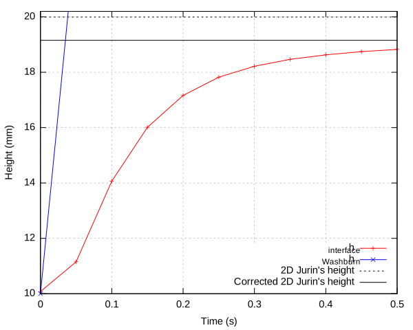
We can see that, here, the gravity is too important to neglect it, even for the transient state. The assumptions made in Washburn’s equation are not valid for this test case.
set grid
set key top right
set xlabel "Time (s)"
set ylabel "Angle (°)"
plot for [i=5:8] sprintf("angle_maxlevel_%d.dat",i) us 1:2 w lp \<div class=message id=243><div id=msg_logo><img src=/img/warning.png></div><div id=msg_label> gnuplot: all points y value undefined!</div></div>
~~~ {.bash}
        title sprintf("nx = %d, dx = %.2e",2**i,2*0.005/2**i), \
        30 w l lc rgb "black" title "Angle imposé"
event end (t = end)
{
  //Interface data
  CapData data = cap_properties (f, cs, beta, R);
  //double V = data.V;

  fprintf(fp4, "============================");
  //Final height of the simulation
  fprintf(fp4, "h_sim = %g mm \n", 1000*data.h_int);

  //Final contact angle
  fprintf(fp4, "theta = %g \n", data.theta_right);

  fclose (fp1);
  fclose (fp2);
  fclose (fp3);
  fclose (fp4);
  fclose(fp5);
}
References
| [asghar_numerical_2025] |
M. H. Asghar, M. Fricke, D. Bothe, and T. Marić. Numerical wetting simulations using the plicRDF-isoAdvector unstructured Volume-of-Fluid (VOF) method. Computers & Mathematics with Applications, 180:191–213, February 2025. [ DOI | http ] |
| [grunding_comparative_2020] |
D. Gründing, M. Smuda, T. Antritter, M. Fricke, D. Rettenmaier, F. Kummer, P. Stephan, H. Marschall, and D. Bothe. A comparative study of transient capillary rise using direct numerical simulations. Applied Mathematical Modelling, 86:142–165, October 2020. [ DOI | http ] |
| [grunding_capillary_2020] |
D. Gründing, M. Smuda, T. Antritter, M. Fricke, D. Rettenmaier, F. Kummer, P. Stephan, H. Marschall, and D. Bothe. Capillary Rise – A Computational Benchmark for Wetting Processes. Applied Mathematical Modelling, 86:142–165, October 2020. [ DOI | arXiv | http ] |
| [grunding_enhanced_2020] |
D. Gründing. An enhanced model for the capillary rise problem. International Journal of Multiphase Flow, 128:103210, July 2020. [ DOI | http ] |
//fixme :see why there is an error for angle's plot