oscillation_3d_ebit.c

3D drop oscillation
- Results
- References

3D drop oscillation

This benchmark has been widely used to assess numerical surface-tension models. In most studies, the Lamb solution, derived from a normal-mode analysis, is used as thereference. The drop oscillation is described as a damped harmonic motion, with oscillation frequency

\omega_n^2 = \frac{n (n + 1) (n - 1) (n + 2) \sigma}{[(n + 1) \rho_1 + n \rho_2] r^3},

and exponentially decaying amplitude a_n(t) = a_0 \exp^{-t/\tau}, \tau = \frac{r_0^2}{(n - 1)(2n + 1)\nu}

However, the motion of a deformed drop initially released from a quiescent velocity field is more accurately described by the Prosperetti solution, which is obtained by solving the corresponding initial-value problem. The Prosperetti solution can be computed using this Python script.

#include "grid/octree.h"
#include "navier-stokes/centered.h"
#include "two-phase-ebit.h"
#include "tension.h"

uf.n[bottom] = 0.;
uf.n[top] = 0.;
uf.n[left] = 0.;
uf.n[right] = 0.;
uf.n[back] = 0.;
uf.n[front] = 0.;

int level = 6, maxlvl, minlvl;
const double R = 1.;
const double EPSR = 0.025;
double la = 1. [0];

double tp_max = 1. [0,1];
double t_step = 1. [0,1];

int main(int argc, char * argv[]) {
  if (argc > 1)
    level = atoi (argv[1]);
  maxlvl = level;
  minlvl = max(level - 5, 3);

  rho1 = 10. [-3,0,1];
  rho2 = 0.1;
  mu1 = 5.e-2;
  mu2 = 5.e-4;

  // f.sigma = 10.;
  f.sigma = 0.1;

  int no = 2;
  double omega2 = no*(no-1)*(no+1)*(no+2)*f.sigma/((no+1)*rho1 + no*rho2)/cube(R);
  double omega = sqrt(omega2);
  la = 2.*rho1*R*f.sigma/sq(mu1);

  tp_max = 2.*2.*pi/omega;

  TOLERANCE = 1e-6 [*];
  CFL = 0.1;

  size (4. [1]);
  origin (-L0/2., -L0/2., -L0/2.);
  init_grid (1 << maxlvl);

  DT = 2.*pi/omega/(1 << 9);
  t_step = DT;
  run();
}

The initial radial position of the droplet interface is r(\theta) = r_0 + \epsilon P_n(\cos \theta) where P_n is the nth-order Legendre polynomial, and the second-order mode is investigated here.

event init (i = 0) {
  vertex scalar phi[];
  foreach_vertex() {
    double cth, dr2, rth, pn;
    dr2 = sq(z) + sq(y) + sq(x);
    cth = z/(sqrt(dr2) + 1.e-32);
    pn = 0.5*(3.*sq(cth) - 1.);
    rth = R + EPSR*pn;
    phi[] = rth - sqrt(dr2);
  }

  char method_name[] = "EBIT";
  init_markers (phi);

  if (pid() == 0)
    printf ("%s R:%g, Sigma:%g, La:%g DT:%.5e\n", method_name, R, f.sigma, la, DT);
}

event logfile (t += t_step; t <= tp_max) {
  double zmax = 0., zmin = HUGE;
  double ke = 0., ke_total = 0.;
  foreach (reduction(+:ke) reduction(+:ke_total)) {
    ke += cube(Delta)*(sq(u.x[]) + sq(u.y[]) + sq(u.z[]))*rho(f[])*f[];
    ke_total += cube(Delta)*(sq(u.x[]) + sq(u.y[]) + sq(u.z[]))*rho(f[]);
  }

  foreach_vertex (reduction(max:zmax) reduction(min:zmin)) {
    if (with_marker.z[] > 0) {
      double zm = z + s.z[]*Delta;
      zmax = max(zmax, zm);
      zmin = min(zmin, zm);
    }
  }
  zmax -= R;
  zmin += R;

  fprintf (stderr, "%.8e %.8e %.8e %.8e %.8e\n", t, zmax, zmin, volume, ke);
  fflush (stderr);
}

Results

The numerical results obtained at \textrm{La} = 800, N_x = 64 are compared with both the Lamb solution and Prosperetti solution.

set term pop
reset
set grid
set ylabel 'a_n/a_0'
set xlabel 't/T_0'
set key bottom right
plot [0:2][-1.1:1.1] 'log' u ($1/22.288):($2/0.025) w l t 'EBIT', \
'../ref_solutions/droplet_ana_800.dat' u ($1/22.288):($2/0.025) w l dt 2 t 'Lamb', \
'../ref_solutions/droplet_ana_800.dat' u ($1/22.288):($3/0.025) w l dt 2 t 'Prosperetti'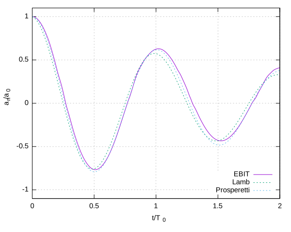

References

[prosperetti1980]	Andrea Prosperetti. Free oscillations of drops and bubbles: the initial-value problem. J. Fluid Mech., 100:333–347, 1980. [ DOI ]
[lamb1932]	Horace Lamb. Hydrodynamics. Dover, 1932.