sandbox/ecipriano/run/dynamic.c
Mesh dependent dynamic contact angle
Moving contact lines are often simulated by combining a static contact angle model with no-slip boundary conditions on the solid surface. However, this combination leads to a singularity in the viscous stresses at the contact line, which is typically regularized by introducing a small slip length (although other regularization mechanisms exist).
In VOF simulations, the interface is advected by the face velocity, located half a grid cell away from the solid boundary. This introduces an implicit (numerical) slip length that removes the contact line singularity. However, this also results in mesh-dependent solutions.
In this file, we implement the models proposed by Afkhami et al. (2009) and Legendre and Maglio (2015). These models exploit a Cox–Voinov-type law to dynamically adjust the contact angle based on the local capillary number.
The two expressions for the dynamic contact angle considered here are:
g(\theta_{d,1}) = g(\theta_s) + Ca_{cl} \log \left(\dfrac{L}{\lambda}\right) \quad \text{with} \quad g(\theta) = \int_0^\theta \dfrac{x - \sin{x}\cos{x}}{2\sin{x}} \, dx
computed using the polynomial fit: \text{g}(x) \approx x^3/9 + 0.00183985x^{4.5} + 1.845823\times 10^{-6} x^{12.258487} \text{g}^{-1}(x) \approx \sqrt[3]{9x} + 0.0727387 x - 0.0515388 x^2 + 0.00341336 x^3
For \theta_d < 3\pi/4 this relation simplifies to (Legendre and Maglio, 2015):
\theta_{d,1}^3 = \theta_s^3 + 9 Ca_{cl} \log\left(\dfrac{L}{\lambda}\right)
For density ratio equal to 1 and |\cos(\theta)| < 0.6 we can use the form proposed by Afkhami et al., 2009:
\cos{\theta_{d,2}} = \cos{\theta_{s}} - 5.63 \, Ca_{cl} \log\left(\dfrac{L}{\lambda}\right)
where the capillary number at the contact line is defined as Ca_{cl} = \mu u_{cl} / \sigma.
The length scale at which the contact angle is resolved is \Delta/2, while the length scale at which the apparent (equilibrium) contact angle belongs depends on the model. Different configurations are summarized in the following table (adapted from Legendre and Maglio, 2015).
| Name | Contact angle | Numerical scale L | Equilibrium angle scale \lambda | Slip length \lambda_N |
|---|---|---|---|---|
| Stat1 | \theta_d = \theta_s | — | — | 0 |
| Stat2 | \theta_d = \theta_s | — | — | \Delta/2 |
| Stat3 | \theta_d = \theta_s | — | — | \Delta_{32}/2 |
| Dyn1 | \theta_d = \theta_{d1} | 10^{-6} | 10^{-9} | 0 |
| Dyn2 | \theta_d = \theta_{d1} | \Delta/2 | 10^{-9} | 0 |
| Dyn3 | \theta_d = \theta_{d1} | \Delta/2 | 10^{-9} | \Delta/2 |
| Dyn4 | \theta_d = \theta_{d2} | \Delta/2 | K=0.04R | 0 |
Sessile droplet
We can see that for each level of refinement, the droplet correctly relaxes towards a steady configuration (the scheme is well-balanced). However, the spreading dynamics changes depending on the resolution: as we increase the refinement we tend toward the no-slip condition, which justifies the slower evolution of the higher refinements.
set size square
set xr[0:1]
set yr[0:1]
set grid

plot "facets-5" u 1:2 w l lw 1.2 lc -1 dt 4 t "LEVEL 5", \
     "facets-6" u 1:2 w l lw 1.2 lc -1 dt 3 t "LEVEL 6", \
     "facets-7" u 1:2 w l lw 1.2 lc -1 dt 2 t "LEVEL 7", \
     "facets-8" u 1:2 w l lw 1.2 lc -1 dt 1 t "LEVEL 8", \
     "facets-9" u 1:2 w l lw 1.2 lc  7 dt 1 t "LEVEL 9"
set term pop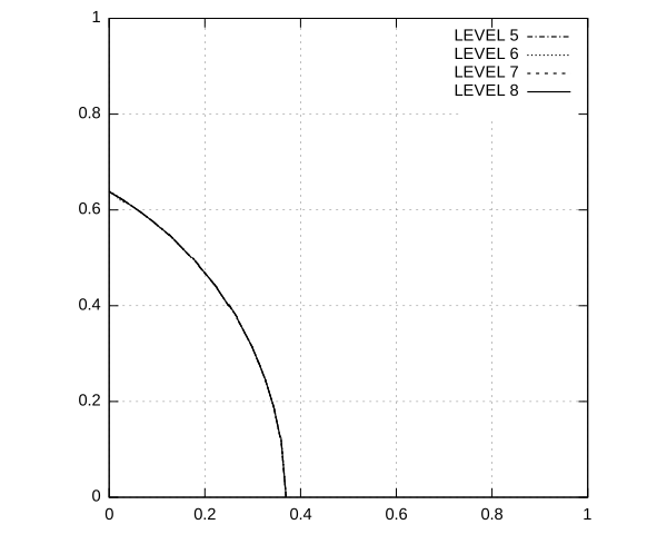
reset
set xlabel "tau [-]"
set ylabel "R/R_0 [-]"
set grid
set key bottom right

plot "<grep 'setup 1 level 5' log" u 5:6 w lp lw 1.2 lc -1 dt 4 t "LEVEL 5", \
     "<grep 'setup 1 level 6' log" u 5:6 w lp lw 1.2 lc -1 dt 3 t "LEVEL 6", \
     "<grep 'setup 1 level 7' log" u 5:6 w lp lw 1.2 lc -1 dt 2 t "LEVEL 7", \
     "<grep 'setup 1 level 8' log" u 5:6 w lp lw 1.2 lc -1 dt 1 t "LEVEL 8", \
     "<grep 'setup 1 level 9' log" u 5:6 w lp lw 1.2 lc  7 dt 1 t "LEVEL 9"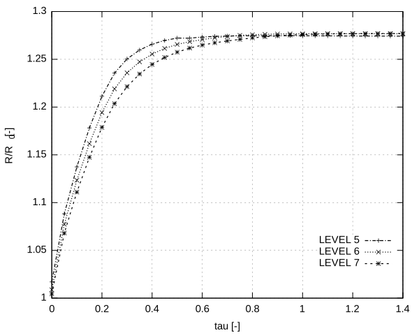
Introducing a Navier slip boundary condition with a slip length smaller than half the grid size (i.e. under-resolved) is effectively equivalent to imposing a no-slip condition in terms of contact line convergence. However, the presence of slip still affects the dynamics, slowing down the interface evolution at all refinement levels compared to the no-slip case.
We can achieve convergence on the interface position by using a slip length which is larger than the grid size. In this case, it is equal to half the size of the coarsest grid. However, if the viable grid refinements are much larger than the physical slip length, this method is not adequate since it introduces too much slip. For example, in the following plots the interface position does converge, but at a much lower elevation compared to the no-slip case.
reset
set xlabel "tau [-]"
set ylabel "R/R_0 [-]"
set grid
set key bottom right

plot "<grep 'setup 3 level 5' log" u 5:6 w lp lw 1.2 lc -1 dt 4 t "LEVEL 5", \
     "<grep 'setup 3 level 6' log" u 5:6 w lp lw 1.2 lc -1 dt 3 t "LEVEL 6", \
     "<grep 'setup 3 level 7' log" u 5:6 w lp lw 1.2 lc -1 dt 2 t "LEVEL 7", \
     "<grep 'setup 3 level 8' log" u 5:6 w lp lw 1.2 lc -1 dt 1 t "LEVEL 8", \
     "<grep 'setup 3 level 9' log" u 5:6 w lp lw 1.2 lc  7 dt 1 t "LEVEL 9"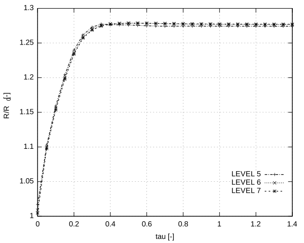
Introducing the dynamic angle models we can enforce the convergence of the spreading dynamics. The model is really sensitive to the way the capillary number and the contact line is computed, and to how the interface position is reconstructed.
reset
set xlabel "tau [-]"
set ylabel "R/R_0 [-]"
set grid
set key bottom right

plot "<grep 'setup 5 level 5' log" every 2 u 5:6 w lp lw 1.2 lc -1 dt 4 t "LEVEL 5", \
     "<grep 'setup 5 level 6' log" every 2 u 5:6 w lp lw 1.2 lc -1 dt 3 t "LEVEL 6", \
     "<grep 'setup 5 level 7' log" every 2 u 5:6 w lp lw 1.2 lc -1 dt 2 t "LEVEL 7", \
     "<grep 'setup 5 level 8' log" every 2 u 5:6 w lp lw 1.2 lc -1 dt 1 t "LEVEL 8", \
     "<grep 'setup 5 level 9' log" every 2 u 5:6 w lp lw 1.2 lc  7 dt 1 t "LEVEL 9"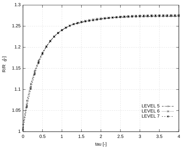
reset
set xlabel "tau [-]"
set ylabel "R/R_0 [-]"
set grid
set key bottom right

plot "<grep 'setup 7 level 5' log" u 5:6 w lp lw 1.2 lc -1 dt 4 t "LEVEL 5", \
     "<grep 'setup 7 level 6' log" u 5:6 w lp lw 1.2 lc -1 dt 3 t "LEVEL 6", \
     "<grep 'setup 7 level 7' log" u 5:6 w lp lw 1.2 lc -1 dt 2 t "LEVEL 7", \
     "<grep 'setup 7 level 8' log" u 5:6 w lp lw 1.2 lc -1 dt 1 t "LEVEL 8", \
     "<grep 'setup 7 level 9' log" u 5:6 w lp lw 1.2 lc  7 dt 1 t "LEVEL 9"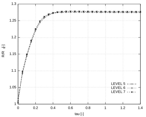
Conclusions
Both the formulation by Afkhami et al. (2009) and the models by Legendre and Maglio (2015) converge, although the results are different.
It is also important to note that a straightforward implementation of these models does not guarantee correct behavior. In particular:
- The interface position should be computed using height functions to ensure accurate contact line dynamics.
- At high levels of refinement, small oscillations in the contact line velocity can induce large variations in the dynamic contact angle, potentially jeopardizing the simulation. To mitigate this issue, we introduce a relaxation factor that limits the variation of the contact angle between consecutive time steps.
- The factor 9 in Legendre and Maglio (2015) can not be omitted if we want to have the same behavior of the polynomial form. There must be a typo in the paper.
Simulation setup
We resolve the Navier–Stokes equations for a two-phase system with surface tension and contact angle.
//#include "grid/multigrid.h"
#include "axi.h"
#include "navier-stokes/centered.h"
#include "contact-small.h"
#include "dynamic.h"
#include "two-phase.h"
#include "tension.h"
#include "reduced.h"

#ifndef MAXLEVEL
# define MAXLEVEL 7
#endif

double theta0 = 60.;
vector h[];
h.t[left] = contact_angle (thetad*pi/180.);

u.n[left] = dirichlet (0.);
u.t[left] = navier (0., SLIP_LENGTH);
p[left] = neumann (0.);

int maxlevel, setup = 0;
double R0 = 0.5, tend = 1.4;

void run_levels (void (* setup_case) (void)) {
  setup++;
  for (maxlevel = 5; maxlevel <= MAXLEVEL; maxlevel++) {
    HALF_COARSE_SIZE = 0.5*L0/(1 << 5);
    HALF_GRID_SIZE = 0.5*L0/(1 << maxlevel);

    setup_case();
    init_grid (1 << maxlevel);
    run();
  }
}

int main (void) {
  rho1 = rho2 = 1.;
  mu1 = mu2 = 0.25;

  f.sigma = 7.5;
  f.height = h;

  run_levels (setup_stat1);
  run_levels (setup_stat3);
  run_levels (setup_dyn4);
  tend = 4.; run_levels (setup_dyn2);
}

#define circle(x,y,R) (sq(R) - sq(x) - sq(y))

event init (i = 0) {
  fraction (f, circle (x, y, R0));
}

#if TREE
event adapt (i++) {
  adapt_wavelet ({f,u.x,u.y}, {1e-2,1e-2,1e-2}, maxlevel);
}
#endif
Post-processing
Using the height functions for computing the interface position gives more accurate results compared to the mycs reconstruction.
event logger (t += 0.05) {
  double xcl = HUGE;
  foreach_boundary (left, serial)
    if (is_contact_x (point, f, theta0*pi/180.))
      xcl = min (xcl, interface_position (point, f));
  double Ca = capillary();

  fprintf (stderr, "setup %d level %d %g %g %g %g\n",
      dyn_setup, maxlevel, t, xcl/R0, Ca, thetad);
}

#if 0
#include "view.h"

event movie (t += 0.01) {
  clear();
  view (tx = -0.5, ty = -0.5);
  draw_vof ("f", lw = 2.);
  squares ("u.y", spread = -1);
  box();
  save ("movie.mp4");
}
#endif

event end (t = tend) {
  char name[80];
  sprintf (name, "facets-%d", maxlevel);
  FILE * fp = fopen (name, "w");
  output_facets (f, fp);
  fclose (fp);
}
References
| [legendre2015] |
Dominique Legendre and Marco Maglio. Comparison between numerical models for the simulation of moving contact lines. Computers and Fluids, 113:2–13, 2015. [ DOI | http | .pdf ] |
| [afkhami2009] |
Shahriar Afkhami, Stephane Zaleski, and Markus Bussmann. A mesh-dependent model for applying dynamic contact angles to vof simulations. Journal of computational physics, 228(15):5370–5389, 2009. [ .pdf ] |