sandbox/easystab/david/differential_equation_infinitedomain.m

Solving a linear differential equation ON AN INFINITE DOMAIN.

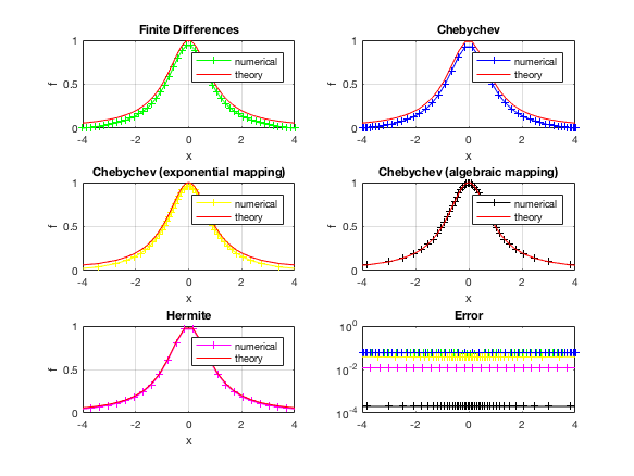
This code will compare five discretization methods for the following problem: \displaystyle \frac{d^2 F}{d x^2} = \frac{6x^2 - 2}{(x^2+1)^3}; \quad F(\infty) = 0 ; \quad F(-\infty) = 0. Whose theoretical solution is : F(x) = \frac{1}{1+x^2}.

We compare the following discretization methods:

• FD on a truncated domain
• Chebychev on a truncated domain (bc. are imposed at x=\pm L with L=4).
• Chebychev with a coordinate mapping (exponential and algebraic)
• Hermite

At the end of the program we will also compare the efficencies of the methods to compute the integral of the function F, whose theoretical value is pi.

    clear all; clf
    % parameters
    N=50; % number of points

    G = @(X)(6*X.^2-2)./(X.^2+1).^3;
    FF = @(X)(1./(1+X.^2));
    Itheo = pi;

Solution with finite elements

The simplest idea is to truncate the domain to a finite one, and use simple finite differences. The main problem will be that the boundary conditions at infinity will have to be imposed at the artificial boundaries.

Here we try this idea for a domain [-4,4]. The results (see figure at the bottom of this program) show some deviation with respect to the theoretical solution.

Of course, we can extend the domain to larger ones (try for instance [-20,20]) but the mesh will become coarse in the central region, unless the number of points (N) is strongly increased. Thus better methods have to be found.

    %% building the differentiation matrices with dif1D:
    [dx,dxx,wx,x]=dif1D('fd',-4,8,N);
    Z=zeros(N,N); I=eye(N);
    %% I build the linear differential equation
    A=dxx;
    Y=G(x);
    
    %% boundary conditions
    A([1,N],:)=[I(1,:); I(N,:)]; 
    Y([1,N])=[0,0];
    
    %% solve the system
    F=A\Y;
   
    %% plotting the results and comparing with theory
    Ftheo = FF(x);
    Error = F-Ftheo;
    subplot(3,2,1)
    plot(x,F,'g-+',x,Ftheo,'r-');
    xlabel('x');ylabel('f');
    legend('numerical','theory')
    xlim([-4,4]); grid on
    title('Finite Differences');
     
    subplot(3,2,6)
    semilogy(x,abs(Error),'g-+');hold on;
    Ifd = wx*Ftheo; % integral

Solution with Chebyshev

We do the same thing with Chebyshev on a truncated domain [-4,4]. This method has the same drawbacks as the previous one.

    %% building the differentiation matrices with dif1D:
    [dx,dxx,wx,x]=dif1D('cheb',-4,8,N);
    Z=zeros(N,N); I=eye(N);
  
     %% I build the linear differential equation
    A=dxx;
    Y=G(x);
    
    %% boundary conditions
    A([1,N],:)=[I(1,:); I(N,:)]; 
    Y([1,N])=[0,0];
   
 %% solve the system
    F=A\Y;
   
%% plotting the results and comparing with theory
    Ftheo = FF(x);
    Error = F-Ftheo;
    subplot(3,2,2)
    plot(x,F,'b-+',x,Ftheo,'r-');
    xlabel('x');ylabel('f');
    legend('numerical','theory')
    xlim([-4,4]); grid on
    title('Chebychev');
     
    subplot(3,2,6)
    semilogy(x,abs(Error),'b-+');
    
    Icheb = wx*Ftheo; % integral

Solution with Hermite polynomials

This method is specifically designed to treat problems in an infinite domain. The idea is to expand the solution over the basis of Hermite functions defined as H_n(x) exp{-x^2} where H_n is the Hermite polynomial of order n. The collocation points (mesh points) are the roots of the largest polynomial used in the expansion, namely H_N(x).

This method does not require to impose boundary conditions because it naturally assumes that the functions to be computed tend to zero as x \rightarrow \pm \infty.

Results (see figure) show good agreement. However, the Hermite method works best of the function decay exponentially as x\rightarrow \infty, which is not the case here.

    %% building the differentiation matrices with dif1D:
    [dx,dxx,wx,x]=dif1D('her',0,1,N);
    Z=zeros(N,N); I=eye(N);
  
     %% I build the linear differential equation
    A=dxx;
     Y=G(x);
    
    %% boundary conditions
    %A([1,N],:)=[I(1,:); I(N,:)]; 
    %Y([1,N])=[0,0];
   
 %% solve the system
    F=A\Y;
   
%% plotting the results and comparing with theory
    Ftheo = FF(x);
    Error = F-Ftheo;
    subplot(3,2,5)
    plot(x,F,'m-+',x,Ftheo,'r-');
    xlabel('x');ylabel('f');
    legend('numerical','theory')
    xlim([-4,4]); grid on
    title('Hermite');
     
    subplot(3,2,6)
    semilogy(x,abs(Error),'m-+');
    xlim([-4,4]);
    title('Error');
    
    Iher = wx*Ftheo; % integral

Solution with Stretched Chebyshev (Algebraic mapping)

The idea is to first define a grid using Chebyshev points for a “reduced coordinate” \xi belonging to a bounded domain [\xi_{min},\xi_{max}], and then to “stretch” this domain to a much larger one [x_{min},x_{max}] by the use of a mapping function x=X(\xi).

The matricial operators \partial_\xi, \partial_{\xi\xi}, etc… for the “reduced variable” are constructed in the usual way using chebdif. The differential operators for the physical variable x are deduced through

\displaystyle \partial_x = \left(\frac{dX}{d\xi}\right)^{-1} \partial_\xi and similar formulas for the higher-order derivatives.

The algebraic mapping, which is found to lead to the best results in most cases, is defined as follows :

\displaystyle X(\xi) = \frac{H \xi}{\sqrt{1-\xi^2}}

This function maps the domain \xi \in [-1,1] to the domain x\in [-\infty,\infty]. In practise, it is preferable to use this \xi \in [-b,b] where b is a parameter smaller than 1. This will map the domain to (x_{min},x_{max}) = Hb/$ which is very large if b is close to 1.

The method requires two parameters : * The factor H is a scaling factor. About half of the grid points will be contained in the domain [-L,L]. * The parameter b controls the stretching (0.999 gives good results).

The construction of the mapping and the differential operators is done in the dif1D.m function by specifying ‘chebInfAlg’ as the first argument.

    %% building the differentiation matrices with dif1D:
    H = 1;b=0.9999;
    [dx,dxx,wx,x]=dif1D('chebInfAlg',0,H,N,b);
    Z=zeros(N,N); I=eye(N);
  
     %% I build the linear differential equation
    A=dxx;
     Y=G(x);
    
    %% boundary conditions
    A([1,N],:)=[I(1,:); I(N,:)]; 
    Y([1,N])=[0,0];
   
 %% solve the system
    F=A\Y;
   
%% plotting the results and comparing with theory
    Ftheo = FF(x);
    Error = F-Ftheo;
    subplot(3,2,4)
    plot(x,F,'k-+',x,Ftheo,'r-');
    xlabel('x');ylabel('f');
    legend('numerical','theory')
    xlim([-4,4]); grid on
    title('Chebychev (algebraic mapping)');
     
    subplot(3,2,6)
    semilogy(x,abs(Error),'k-+');
    
    IchebInfAlg = wx*Ftheo; % integral    

Solution with stretched Chebyshev (exponential mapping)

The method of “coordinate stretching” can be employed using other choices of functions.

Here we give an example with the “exponential mapping” defined by

\displaystyle x = X(\xi) = \tanh(\xi)

    %% building the differentiation matrices with dif1D:
    [dx,dxx,wx,x]=dif1D('chebInfExp',0,1,N,0.9999);
    Z=zeros(N,N); I=eye(N);
  
     %% I build the linear differential equation
    A=dxx;
     Y=G(x);
    
    %% boundary conditions
    A([1,N],:)=[I(1,:); I(N,:)]; 
    Y([1,N])=[0,0];
   
 %% solve the system
    F=A\Y;
   
%% plotting the results and comparing with theory
    Ftheo = FF(x);
    Error = F-Ftheo;
    subplot(3,2,3)
    plot(x,F,'y-+',x,Ftheo,'r-');
    xlabel('x');ylabel('f');
    legend('numerical','theory')
    xlim([-4,4]); grid on
    title('Chebychev (exponential mapping)');
     
    subplot(3,2,6)
    semilogy(x,abs(Error),'y-+');
    
    IchebInfExp = wx*Ftheo; % integral
    

    
    set(gcf,'paperpositionmode','auto')
    print('-dpng','-r75','differential_equation_infinite.png')

Computing an integral

    disp(' Computing the integral :') 
    Itheo    
    Ifd
    Icheb
    IchebInfExp
    IchebInfAlg
    Iher

The results

Exercice :

Modify the code to compare the various methods for the differential problem :

\displaystyle \frac{d^2 F}{d x^2} = (4 x^2-2 ) e^{-x^2} ; \quad F(\infty) = 0 ; \quad F(-\infty) = 0.

Whose theoretical solution is : F(x) = e^{-x^2} (with I = \sqrt{\pi}).

%