**(This document belongs to the lecture notes for the [M2-DET](http://basilisk.fr/sandbox/easystab/M2DET/Instabilities.md) course, D. Fabre, nov. 2018-dec. 2023)**


This documents gives mathematical support for the study of dynamical systems (lectures 1-2 of the course)

<span style="color:green">
Paragraphs in green can be skipped at first lecture.
</span>

# Introduction and General definitions 

- A *dynamical system* (DS) of order $N$ is by definition a system of $N$ order-one ordinary differential equations (ODEs) 
written as follows : 
$$
\frac{d X}{dt} = F(X,t)
$$
where $X(t) = [x_1(t);x_2(t);x_3(t); ... x_N(t)]$ is a N-dimensional state variable belonging to the *phase space*   $\mathbb{R}^N$, and $F(X,t) = [f_1(x_1,x_2, ...,t);f_2(x_1,x_2, ...,t);... f_N(x_1,x_2, ...,t) ]$.

- <span style="color:green"> Remark: Dynamical systems are a particular cases of "algebraic differential systems" with the form $E \frac{d X}{dt} = F(X,t)$ where $E$ is a non-invertible matrix. Such systems are encountered in cases where we have both dynamical equations and constraints. In most cases algebraic differential systems can actually be treated as dynamical ones.
</span>

- The dynamical system is said to be *autonomous* if $F(X,t)=F(X)$.  

- The function $F(X,t)$ is called the *flow* of the DS. 

- A *trajectory* in the phase space is defined by the curve $X(t)$ corresponding to the solution of the system corresponding to a given initial condition (i.e. the speficifation of $X(t=0) = X_{init}$).

- A *fixed point* or *equilibrium point* of an autonomous DS is a point $X=X^0$ such as $F(X^0) = 0$. It is thus a particular type of trajectory reduced to a single point.

- A *cycle* is a closed trajectory in the phase-space.

- A *phase portrait* is a graphical representation of a selection of trajectories of the DS (including the most significant ones such as fixed points, limit cycles, etc...).

Rather than focusing on individual trajectories corresponding to specific initial conditions, the general idea of DS theory is 
to consider the dynamics of the system from a global point of view by investigating the *flow* in the *phase space* in a geometrical and topological way. 







### Illustration : the pendulum

( use program [PhasePortrait_NonLinear.m](/sandbox/easystab/PhasePortrait_NonLinear.m) 


### Conservative vs. non-conservative systems

In the framework of DS theory, a system is said to be *conservative* if the flow verifies $div(F) = \partial f_i / \partial x_i$ = 0. If not ot is called *non-conservative*.

Non-conservative systems generally possess *contracting regions* of the phase-space in which $div(F)<0$. If the whole phase-space is contracting, then the system itself is called a *contracting system*. Sometimes the term *dissipative system* is employed as a synonymous (but it is better to avoid this term, as explained above).

A geometrical interpretation of the property $div(F) <0$ is that trajectories originating from close points tend to approach each others. 
As a consequence, in contracting regions the trajectories converge towards specific parts of the phase-space called *attractors*. The most simple kinds of attractors are fixed points and *limit cycles*, but other kind can be encountered, including very unexpected ones called *strange attractors* (see lecture 5).

Conservative systems are usually encountered in idealised cases. In such systems, phase portraits do not display attractors, but may contain a continuous set of cycles, and possibly *heteroclinic connections* joining the fixed points (illustration for the conservative pendulum).


### Remark : Dynamical systems vs. Hamiltonian systems

<span style="color:green">
The formalism of Dynamical systems is close to the one of Hamiltonian mechanics. However, there is a important difference. 
In Hamiltonian mechanics, a Hamiltonian system is defined by the state-vector 
$X = [x_1(t), x_2(t), ... x_N(t) ;  \dot{x}_1(t), \dot{x}_2(t), ... \dot{x}_N(t)]$. Hence, a hamiltonian system of order $N$ corresponds to a dynamical system of order $2N$.


### Remark on conservative/dissipative notions.

<span style="color:green">
The definitions of a conservative system given above is mathematical one, somewhat different from the usual definition of a conservative physical system. 
A physical system is called *conservative* if there exists a invariant function "Energy" $E(X)$ such as $dE/dt=0$. Another, practically equivalent definition is that the system is *time-reversible*. These physical definitions are not always equivalent to the mathematical one given here. 

<span style="color:green">
Similarly, a physical system is called *dissipative* if $dE/dt < 0$ (implying that it is not time-reversible). This definition has to be distinguished from the mathematical definition of a contracting DS, and the two cases do not always overlap. For instance, modelling of a dissipative physical system by a low-order model may lead to a DS which is not contracting ! (See lecture 5.)


<span style="color:green">
On the other hand, the two definitions of *conservative* turn out to be equivalent for the important case of two-dimensional systems ($N=2$), as one can show that a conservative two-dimensional system is always associated to an energy (it is *integrable*).
</span>



# Stability of fixed-points of a dynamical system (Lecture 1)

## Definitions

- A fixed point $X^0$ is said to be *stable* if there exists a neighborhood $\Omega_0$ of $X^0$ such that $X(t) \rightarrow X_0$ for all initial conditions $X(t=0) \in \Omega_0$ .


- <span style="color:green"> A fixed point is said to be *exponentially stable* (or *linearly stable*) if it is stable and verifies the additional condition : $||X(t)-X^0|| \leq C e^{-\gamma t}$ for some positive constants $\gamma$ and $C$.


- <span style="color:green"> A fixed point is said to be *monotonically stable* if it is stable and verifies the additional condition : $d||X-X^0||/dt \leq 0$ for all initial conditions $X(t=0) \in \Omega_0$ .

- A fixed point $X^0$ is said to be *unstable* if there exists at least one trajectory starting from an initial condition arbitrarily close to $X^0$ and diverging from this point.

## Linearization of a dynamical system in the neighborhood of a fixed point. 

The general method  for studying the stability properties of a fixed-point consists of  *Linearizing* the DS in the vicinity of the fixed-point.

For this we consider small-amplitude perturbations by assuming:

$$
X = X^0 + \epsilon X'(t)
$$

Then a Taylor expansion leads to :

$$
\frac{ d X'}{dt } + A X' + \mathcal{O}( \epsilon)  
$$

Where $A$ is the *Jacobian matrix* or the DS :

$$ 
A = \left[ \nabla  F  \right]_{X^0} \qquad ( \mathrm{ i.e. } A_{ij} = [ \partial f_i / \partial x_j ])
$$

Assuming $\epsilon \ll1$, we can neglect the higher-order terms (*nonlinear terms*). We can thus replace the system by a linear one which is much easier to study. 

## Eigenvalue analysis

*(In the two next sections we assume that the fixed point is at the origin, i.e. $X^0 = 0$ and $X \equiv X'$.)*

Except in "exceptional cases", the solution of the problem can be written as follows:

$$ 
X(t) = \sum_{\lambda_n \in {\mathcal Sp}} c_n \hat X_n e^{\lambda_n t} \qquad \mathrm{ (Eq. 1)}
$$

where  $\lambda_n$ are the *eigenvalues* and the corresponding 
$\hat{X}_n$ the *eigenvectors*. 
The latter are solutions of the eigenvalue problem:
$$
\lambda \hat{X} = A \hat{X}
$$

We supose that the eigenvalues are sorted in the order of decaying real part, namely
$$
Re(\lambda_1) \geq  Re(\lambda_2) \geq  ... \geq  Re(\lambda_N)
$$


According on the eigenvalues we are in one of the three following cases:

- The system is *linearly unstable* if there is at least one eigenvalue with positive real part, namely : if $Re(\lambda_1)>0$

- Reversely, the system is *linearly stable*  if all eigenvalues have negative real part, namely : if $Re(\lambda_1)<0$.

- If $Re(\lambda_1)=0$ the linear system is said to be *marginally stable*. In this case it is necessary to consider the nonlinear terms to decide the stability.

<span style="color:green">
Note that if $A$ is symmetric (or hermitian), the condition for stability implies monotonous stability. If $A$ is nonsymmetric, on the other hand, the system may be exponentially stable but not monotonously stable. This situation corresponds to "transient growth" and will be reviewed in lecture 9.


A more complete document on linear systems of order $N$ can be found [here](http://basilisk.fr/sandbox/easystab/david/LinearSystems.md#linear-dynamical-systems). In the sequel of this document we restrict to the case of 2-dimensional dynamical systems ($N=2$).


## Classification of fixed points in two dimensions


A 2x2 system can be written as follows :

$$
\frac{d}{dt}
\left[ \begin{array}{c} 
x_{1}  \\ x_{2}  
\end{array}
\right] 
= 
\left[ \begin{array}{cc} 
A_{11} & A_{12} \\ A_{21} & A_{22} 
\end{array}
\right]  
\left[ \begin{array}{c} 
x_{1}  \\ x_{2}  
\end{array}
\right] 
$$

We look for the eigenvalues/eigenvectors by solving the eigenvalue problem : $A \hat{X} = \lambda \hat{X}$.

If $\lambda_1$ and $\lambda_2$ are distinct, the solution of this problem can be expressed in terms of the eigenvalues/eigenvectors, as follows :

$$ 
X(t) = c_1 \hat X_1 e^{\lambda_1 t} + c_2 \hat X_2 e^{\lambda_2 t}
$$

According to the values of $\lambda_1$, $\lambda_2$, the fixed point will be called:

- An **unstable node** (noeud instable) if $(\lambda_1,\lambda_2) \in \mathbb{R}^+$.

- A **stable node** (noeud stable) if $(\lambda_1,\lambda_2) \in \mathbb{R}^-$.

- A **saddle** (point-selle, ou col) if $\lambda_1 \in \mathbb{R}^+$, $\lambda_2 \in \mathbb{R}^-$.

- An **unstable focus** (foyer instable) if $\lambda_{1,2} = \sigma \pm i \omega$, $\sigma >0$.

- A **stable focus** (foyer instable) if $\lambda_{1,2} = \sigma \pm i \omega$, $\sigma <0$.

<span style="color:green">
In addition to these five main cases, a number of exceptional cases can be distinguished:


- <span style="color:green"> The case  $\lambda_{1,2} = \pm i \omega$ is called a **center**.


- <span style="color:green"> The case $\lambda_1=0$, $\lambda_2 < 0$ is called a **non-hyperbolic point of dimension 1**. 


- <span style="color:green"> The cases $\lambda_{1}=\lambda_{2} \ne 0$ are called **improper nodes** (stable or unstable).

- <span style="color:green"> (the case $\lambda_{1}=\lambda_{2}=0$ is called a Takens-Bogdanov codimension-two bifurcation point and is even more exceptionnal than the previous ones).


In the two first cases, it is necessary to include nonlinear terms to conclude for stability/instability.
 
**Exercice :**
Study the possible types of fixed points in 2D using the program 
[PhasePortrait_Linear.m](/sandbox/easystab/PhasePortrait_Linear.m) 
 
 
### Map of all possible cases


$\lambda_1$ and $\lambda_2$ are the solutions of the characteristic polynomial $det (A - \lambda I) =0$ which can 
also be written as follows :

$$ 
\lambda^2 - tr (A) \lambda  + det(A) = 0
$$ 

One can classify the various cases in the plane $tr(A)$-$det(A)$, leading to th following diagram (**Exercice**):

![Classification of fixed-points in 2-dimensional systems](/sandbox/easystab/FixedPoints.jpg)

<span style="color:green">
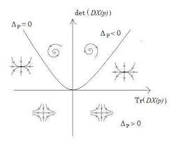
**Remark**: For the case of conservative systems, $det(F) = Tr(A)=0$, hence fixed points are necessarily either *centers* or *saddles* (illustration for the case of the ideal pendulum).

# Exercices for lecture 1

## 1.1. Linear harmonic oscillator

Consider the damped harmonic oscillator, with the form :
$$m \ddot x = - k x - \mu \dot x$$

   a. Write this problem under the form of a linear dynamical system of order 2, considering the state-vector $X = [x,\dot x]$.
   b. Give the nature of the fixed-point $[0,0]$ as function of the parameters (node, focus, etc...)
   c. Explain the correspondance between the identified cases and the classical analysis of this equation (pseudo-pediodic, periodic,  critical,  aperiodic and unstable régimes) 
   c. Using the program [/sandbox/easystab/PhasePortrait_Linear.m](PhasePortrait_Linear.m), draw phase portraits for this problem for the five regimes of solution.

## 1.2. Brusselator 

[Correction](http://basilisk.fr/sandbox/easystab/Correction_Exercices.md#exercice-1.2)


Consider the "Brusselator" 2D dynamical system:

$$\frac{dx}{dt} = A + x^2 y - (B+1) x$$

$$\frac{dy}{dt} = B x-x^2 y $$

This dynamical system is a classical model initially inttroduced to model an oscillating chemical reaction. Here $x$(t) and $y(t)$ correspond to the concentrations of two chemical products, and $A$ and $B$ are constants.


a. Show that this system admits a unique equilibrium point $[x,y] = [x^{(0)},y^{(0)}]$.

b. Study the linear stability of this equilibrium point. Specify the nature of this point (node, focus, ...) as function of the parameters.

## 1.3. 2D model system with two fixed points

Consider the following 2D dynamical system:

$$\frac{dx}{dt} = (1-x) x$$

$$\frac{dy}{dt} = (2-4x) y $$

a. Find the equilibrium points of the system.

b. Determine their nature (stable/unstable, node/saddle/foci...)

c. Draw a phase portrait of this system (you may use the program [/sandbox/easystab/PhasePortrait_NonLinear.m](PhasePortrait_NonLinear.m)).

## 1.4. Linear problem modelling thermal conduction (preparation for chapter 5)

Consider the following dynamical system of order 2 defined as 
$$\frac{d}{d t} X
= A X
$$
with
$$
A = \left[ \begin{array}{cc} 
-\nu k^2  & \alpha g  \\ \beta & - \kappa k^2
\end{array}
\right].
$$

where all quantities $\nu,k,\alpha...$ are real, positive parameters.

a. Write down the trace and determinent of the matrix, and its characteristic polynomial.

b. Discuss, as function of the parameters, the possible behaviours of the system referring to the ($tr(A) - det(A)$) diagram presented in this lecture.

c. Deduce that the fixed point $(0;0)$ is unstable if $\alpha \beta g > \nu \kappa k^4$.  

# Bifurcations (Lecture 2)

## Definitions 

We consider an autonomous system depending upon a *control parameter* r, as follows:

$$
\frac{d X}{dt} = F(X,r)
$$


Definitions : 

- A bifurcation is a qualitative modification of the behaviour of a system occuring for a specific value $r=r_c$, generally associated to a modification of the number of fixed points and./or limit cycles, and a change of their stability properties.

- A *fixed-point bifurcation* occurs if for $r=r_c$ at least one eigenvalue of the Jacobian matrix of the corresponding fixed point has zero real part. 

In other words, when changing the parameter $r$, at least one eigenvalue crosses the imaginary axis in the complex $\lambda$-plane when $r=r_c$.

- We call a *bifurcation diagram* a representation of the amplitude (with a convenient definition) of the fixed-point solutions (and possibly limit cycles) as function of the control parameter. By convention, stable solutions will be represented with full lines, and unstable ones with dashed lines.

### Illustrations (practical work)

Using programs [PhasePortrait_NonLinear.m](/sandbox/easystab/PhasePortrait_NonLinear.m) and 
[PhasePortrait_NonLinear.m](/sandbox/easystab/PhasePortrait_NonLinear.m), build the bifurcation diagrams of the following problems:
- Rotating pendulum
- Inverted pendulum
- Brusselator


# Mathematical analysis of fixed-point bifurcations

## Definitions 

- The *dimension* $n_b$ of a bifurcation is the number of eigenvalues which cross the imaginary axis for $r=r_c$. The generic cases are $n_b = 1$ (one real eigenvalue) and $n_b = 2$ (a pair of complex eigenvalues). All other cases are exceptional (or "codimension-2") and not considered here. 

- The *central manifold* is a geometrical manifold of dimension $n_b$ on which all trajectories in the vicinity of the bifurcation point "relax rapidly" and then "slowly evolve" along it. 
One can justify that this manifold is tangent to the subspaces generated by the nearly-neutral eigenmodes of the fixed points.   

- The *normal form* of a bifurcation is a generic DS of dimension $n_b$ describing the dynamics along the central manifold, to which each type of bifurcation can be reduced by a series of "elementary" mathematical manipulations (change of variables, etc ...).


## One-dimensional bifurcations

One-dimensional bifurcation are the one associated to a single real eigenvalue. The central manifold is a line and the dynamics can be reduced to a one-dimensional equation in terms of a curvilinear coordinate $x$ along the manifold :

$$dx/dt = f(x;r)$$ 

It is convenient to introduce the *potential* function $V(x)$ such that $f(x) = -dV/dx$. Hence the fixed points of the function $f(x)$ corresponds to extremums of the potential. One can demonstrate that stable fixed points are minimums and unstable ones are maximums.

### The pitchfork bifurcation

<span style="color:blue">
Illustration by a physical example :  **The rotating pendulum**. 
See exercice 2.2 and play with the program [PhasePortrait_NonLinear.m](/sandbox/easystab/PhasePortrait_NonLinear.m) ! 
</span>

The *normal form* of a pitchfork bifurcation occuring at $r_c = 0$ is :

$$
dx/dt = f(x;r) = r x - s x^3 \quad \mathrm{ with } \quad s = \pm 1.
$$

If $s=1$ the bifurcation is *supercritical* and for $r>0$ there exist two stable solutions. On the other hand if $s=-1$ the bifurcation is *subcritical* and no stable solution exist for $r>0$ (on the other hand two unstable solutions exist for $r<0$).

The pitchfork bifurcation is generic to systems admitting a spatial (reflexion) symmetry.

### The saddle-node bifurcation

<span style="color:blue">
Illustration by a physical example :  **The inverted pendulum**. 
Play with the program [PhasePortrait_NonLinear.m](/sandbox/easystab/PhasePortrait_NonLinear.m) ! 
</span>

The *normal form* of a saddle-node bifurcation occuring at $r_c = 0$ is :

$$
dx/dt = f(x;r) = r - x^2
$$

This bifurcation is a "fold" connecting two branches of fixed-point solutions. One of them is stable (typically a node) and the other one is unstable (typically a saddle).

### The transcritical bifurcation

<span style="color:blue">
Illustration by a physical example :  **The Buffalo-Wolf system**. 
See exercice 2.3 and play with the program [PhasePortrait_NonLinear.m](/sandbox/easystab/PhasePortrait_NonLinear.m). You should observe two successive transcritial bifurcations for $r=0$ and for $r\approx 0.51$ ! 
</span>

The *normal form* of a transcritical bifurcation occuring at $r_c = 0$ is :

$$
dx/dt = f(x;r) = r x - x^2.
$$

This bifurcation corresponds to the exchange of stability of two fixed-point solutions. It is much less comon in fluid dynamics.


## two-dimensional bifurcations

Two-dimensional bifurcations include the *Hopf bifurcation* (a pair of complex conjugate eigenvalues cross the imaginary $\lambda$-axis for $r=r_c$), and the *Takens-Bogdanov* bifurcation (two zero eigenvalues exist for $r=r_c$). The latter case is exceptionnal (or "codimension-two") so we only consider the first.

### Hopf bifurcation

<span style="color:blue">
Illustration by a physical example :  *The Brusselator *. 
See exercice 1.2 and play with the program [PhasePortrait_NonLinear.m](/sandbox/easystab/PhasePortrait_NonLinear.m) ! 
</span>

If a dynamical system admits a Hopf bifurcation, it is generally possible to reduce it by a series of variable changes to the *Van der Pol* equation 
(which is not exactly a "normal form" in the mathematical sense, but a physically significant model).


$$
\ddot x  + \omega_0^2 x  = (r - s x^2) \dot x \quad \mathrm{ with } \quad s = \pm 1.
$$

- If $s=+1$ the bifurcation is supercritical and a stable limit cycle exists for $r>0$.

- If $s=-1$ the bifurcation is subcritical and an unstable limit cycle exists for $r<0$.

Perturbation methods allow to predict the solution for $r\ll 1$ (averaging method ; multiple-scale methods).


# Exercices for Lecture 2

## 2.1. (Charru, exercice 11.7.12) 

Build the bifurcation diagram of the following amplitude equation, where $\mu$ is the bifurcation parameter:
$$
\frac{d x}{d t} = 4 x ( (x-1)^2-\mu-1 )
$$

Verify that the bifurcation diagram is the one given in figure 11.20 of Charru. (warning : there is a little error in the book ! will you find it ???)

## 2.2. Bifurcation analysis of the rotating pendulum

[Correction](http://basilisk.fr/sandbox/easystab/Correction_Exercices.md#exercice-2.2)


Consider a pendulum with mass $m$ length $L$. The pivot is characterized by a friction coefficient $\mu_f$. The pendulum is in a uniformly rotating frame with rotation rate $\Omega$ with vertical axis.

a. Show that the motion of the pendulum is driven by the following equation :
$$
 m L^2 \ddot \theta = - \mu_f \dot \theta - m g L \sin \theta + m L^2 \Omega^2 \sin \theta \cos \theta 
$$

b. Using convenient nondimensionalization (including redefinition of the time-scale), and under the hypothesis of small angles, show that the equation can be reduced to the "two-dimensional pitchfork equation":
$$
 \ddot x + \dot x = r x  - x^3 
$$
where 
$$ 
r = \frac{m^2 ( \Omega^2 L^4 - g L^3) }{\mu_f^2}
$$

c. Compute the equilibrium points of this equation, and show that they are identical to those of the classical one-dimensional Pitchfork bifurcation. 

d. Study the linear stability of the equilibrium points and give their nature.
Show that a bifurcation occurs for $r=0$ and that a qualitative change of the nature of the equilibrium points occurs for $r=-1/4$ and for $r=1/8$.

(this question may be treated either by calculus of by using the PhasePortrait_NonLinear.m program) 

## 2.3. Buffalo-Wolf system

Using programs [PhasePortrait_NonLinear.m](/sandbox/easystab/PhasePortrait_NonLinear.m), build the bifurcation diagram of the buffalo-wolf system :

$$
\frac{d x_1}{dt} = r x_1 -A x_1 (x_2+E x_2^2) - B x_1^2,
$$
$$
\frac{d x_2}{dt} = -C x_2 + D x_1 (x_2+E x_2^2). 
$$

This systems models the evolution of a two-species ecological system, where $x_1(t)$ is the population of buffaloes and $x_2(t)$ is the population of wholves. 

Here $r$ is the availability of fresh grass (source term for buffaloes), $B$ is the competion between buffalows, $A$ is the predation rate by wholves, $C$ is the rate of death of wholves in absence of buffalows, $D$ is the growth rate of wolves by predating buffaloes, and $E$ is the increase of efficiency of predation due to collaboration between wholves (hunting is more efficient when wholves act in group).  

One will chose the following values :
   
$$
A = .3; B = 0.1; C = 1; D = .2; E = 0.15; F = 0.15
$$ 

and consider $r$ as the bifurcation parameter.


## 2.4. Second-order phase transition (Charru, exercice 1.6.4) 

Consider the following equations, which may be used to model phase transitions in thermodynamics :
$$
\frac{dA}{dt} = -V'(A), \mathrm{ with } V(A) = \mu \frac{A^2}{2} - \alpha \frac{A^4}{4} - \frac{A^6}{6}
$$

a. Justify that stable and unstable points respectively correspond to minima and maxima of the potential function $V(A)$.

b. Draw the potential $V(A)$ for various values of the bifurcation parameter $\mu$. 

c. Deduce a bifurcation diagram of the problem.



## 2.5. Charru, exercice 11.7.11. 

Build the bifurcation diagram of the following amplitude equation, where $\mu$ is the bifurcation parameter: 
$$
\frac{d x}{d t} = x (x^2+\mu)(x^2+\mu^2-1)
$$
 

## 2.6. Charru, exercice 11.7.13. 



 Consider the dynamical system defined as follows :
 
$$
\frac{d}{d t} \left[ \begin{array}{c} x_1 \\ x_1 \end{array} \right] 
= 
\left[ \begin{array}{c} r x_1 - x_1^3 -3  x_2^2 x_1 \\ 
(r-1) x_2 + x_1^2 x_2 - x_2^3 \end{array} \right] 
$$

where $r$ is a control parameter.  




a. Using the program  [/sandbox/easystab/PhasePortrait_NonLinear.m](), draw phase portraits for various values of $r$. 

b. Study the number of fixed points and their stability as function of $r$.

c. Regroup the results under the form of a bifurcation diagram showing the amplitude parameter $A= |x_1|+|x_2|$ of all solutions as function of $r$.