# Andrés Castillo
My name is [Andrés](https://orcid.org/0000-0003-2175-324X).
I store in this location some of the work done in Basilisk. I mainly work with parametric instabilities, vortex instabilities and thermal convection.
# Structure of this sandbox
This sandbox is divided in different parts:
## Vortex Filament Method
This includes an implementation of a Vortex Filament Method (VFM) using [Biot-Savart](filaments/biot-savart.h) and some examples:
* Motion of a [vortex ring](filaments/test_vortex_ring1.h)
* Motion of [2 vortex rings](filaments/test_2vortex_rings1.h)
* Motion of [3 vortex rings](filaments/test_3vortex_rings1.h)
* Motion of an [elliptical vortex ring](filaments/test_vortex_ellipse1.h)
(width=100%)
(width=100%)
(width=100%)
## Output fields
This includes a series of routines to write the resulting fields into several
different formats.
* [output_vtu()](output_fields/vtu/output_vtu.h) - This format is
compatible with the VTK XML file format for unstructured grids [File formats
for VTK version
4.2](http://www.vtk.org/wp-content/uploads/2015/04/file-formats.pdf) which can
be read using Paraview. Here, the results are written in raw binary. The
unstructured grid is required to write results from quadtrees and octrees.
If used in MPI, each MPI task writes its own file, which may be
linked together using a `*.pvtu` file. An example is available
[here](output_fields/vtu/test_output_vtu.c).
* [output_xmf()](output_fields/xdmf/output_xdmf.h) This routine is compatible with the
[XDMF Model and Format](http://www.xdmf.org/index.php/XDMF_Model_and_Format)
which can be read using Paraview or Visit. Data is split in two categories:
*Light* data and *Heavy* data. Light data is stored using eXtensible Markup
Language (XML) to describe the data model and the data format. Heavy data is
composed of large datasets stored using the Hierarchical Data Format
[HDF5](https://support.hdfgroup.org/HDF5/). As the name implies, data is
organized following a hierarchical structure. HDF5 files can be read without
any prior knowledge of the stored data. The list of software capable of
reading HDF5 files includes Visit, Paraview, Matlab, and Tecplot, to name a
few. The type, rank, dimension and other properties of each array are stored
inside the file in the form of meta-data. Additional features include support
for a large number of objects, file compression, a parallel I/O implementation
through the MPI-IO or MPI POSIX drivers. Using this format requires the HDF5
library, which is usually installed in most computing centers or may be
installed locally through a repository. Linking is automatic but requires the
environment variables HDF5_INCDIR and HDF5_LIBDIR, which are usually set when
you load the module hdf5. An example is available
[here](output_fields/xdmf/test_output_xmf.c).
* For testing the XDMF format try:
~~~ { .bash }
sudo apt install libhdf5-dev hdf5-helpers hdf5-tools
export HDF5_INCDIR=/usr/include/hdf5/serial
export HDF5_LIBDIR=/usr/lib/x86_64-linux-gnu/hdf5/serial
make test_output4.tst
~~~
* For testing using MPI try:
~~~ { .bash }
sudo apt install libhdf5-mpi-dev hdf5-helpers hdf5-tools
export HDF5_INCDIR=/usr/include/hdf5/openmpi
export HDF5_LIBDIR=/usr/lib/x86_64-linux-gnu/hdf5/openmpi
CC='mpicc -D_MPI=4' make test_output4.tst
~~~
* After the simulation, it is possible inspect the contents of the *Heavy* data
from the terminal using:
~~~ { .bash }
>> h5ls -r fields.h5
/ Group
/000000 Group
/000000/Cell Group
/000000/Cell/T Dataset {512, 1}
/000000/Cell/pid Dataset {512, 1}
/000000/Cell/u.x Dataset {512, 3}
/000000/Geometry Group
/000000/Geometry/Points Dataset {900, 3}
/000000/Topology Dataset {512, 8}
...
~~~
* [output_vtkhdf()](output_fields/vtkhdf/output_vtkhdf.h) This routine is
compatible with the [VTKHDF File
Format](https://docs.vtk.org/en/latest/design_documents/VTKFileFormats.html#vtkhdf-file-format)
which can be read using Paraview or Visit. VTK HDF files start with a group
called `VTKHDF` with two attributes: `Version`, an array of two integers and
`Type`, a string showing the VTK dataset type stored in the file --- in our case
`UnstructuredGrid`. The data type for each HDF dataset is part of the dataset
and it is determined at write time. In the diagram below, showing the HDF file
structure for `UnstructuredGrid`, the rounded blue rectangles are HDF groups and
the gray rectangles are HDF datasets. Each rectangle shows the name of the group
or dataset in bold font and the attributes underneath with regular font. In our
case, `scalar` and `vector` fields are stored as `CellData`. The unstructured
grid is split into partitions, with a partition for each MPI rank.
An example is available
[here](output_fields/vtkhdf/test_output_vtkhdf.c) and
[here](output_fields/vtkhdf/test_output_vtkhdf2.c).
## Input fields
This includes a series of routines to read existing results and use them as
initial conditions for a new simulation.
* [input_matrix()](input_fields/auxiliar_input.h) - This format reads a binary
file written using [output_matrix()](http://basilisk.fr/src/output.h) and loads
it into a field selected by the user. For instance, to read a square field of
size **L0** defined inside a regular Cartesian grid with **N** points,
starting from (**X0**,**Y0**) stored in a file "example.bin" and load it into
a scalar field,
~~~ {.c}
scalar T[];
...
fprintf (stderr, "Reprising run from existing initial conditions ... \n");
fprintf (stderr, "Read from example.bin ... \n");
FILE * fp = fopen("example.bin", "r");
if (!fp) printf("Binary file not found");
input_matrix(T,fp,N,X0,Y0,L0);
fclose (fp);
...
boundary(T);
~~~
An example on how to generate some arbitrary initial condition using matlab is
available [here](input_fields/test_input_matrix.c)
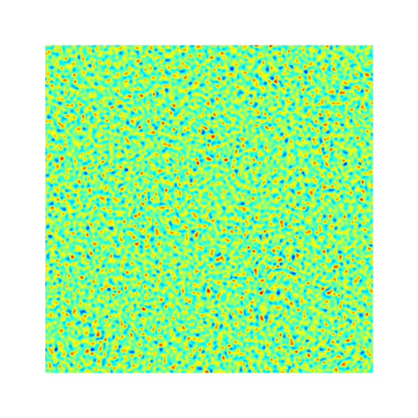
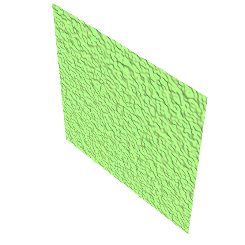
* [initial_condition_2Dto3D()](input_fields/initial_conditions_2Dto3D.h) - This
function reads 2D simulation results from a binary file in a format compatible
with the gnuplot binary matrix format in double precision, see
[auxiliar_input.h](auxiliar_input.h). The 2D results are then used to initialize
a 3D simulation, which may be useful to reduce computational cost by avoiding
long transients, or to focus on the development of 3D instabilities from a 2D
base state.
An example of the intial condition in 2D (left)
and the corresponding 3D interface (right).
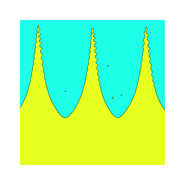
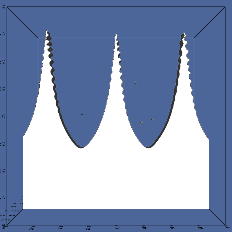
* [initial_conditions_dimonte_fft2()](input_fields/initial_conditions_dimonte_fft2.h)
This can be used to initialize an interface using an annular spectrum as in
[Dimonte et al. (2004)](#dimonte2004).
An example of the initialized interface using `isvof=0` (left)
and `isvof=1` (right).
*****
/**
# Articles Submitted or in Preparation
## Parametric instabilities
~~~bib
@Article{Castillo2025,
author={Andrés Castillo-Castellanos and Benoît-Joseph Gréa and Antoine
Briard and Louis Gostiaux},
title={Mixing induced by Faraday surface waves},
journal={In preparation for Journal of Fluid Mechanics},
year={2025}
}
@Article{Grea2025,
author={Benoît-Joseph Gréa and Andrés Castillo-Castellanos and Antoine
Briard and Alexis Banvillet and Nicolas Lion and Catherine Canac and Kevin
Dagrau and Pauline Duhalde},
title={Frozen waves in the inertial regime},
journal={Submitted to Journal of Fluid Mechanics},
year={2025}
}
~~~
# Articles in Publication
## Vortex flows
~~~bib
@hal{abraham2022, hal-04281239v1}
@hal{castillo2022, hal-03746533v1}
@hal{castillo2021, hal-03401563}
~~~
## Thermal convection
~~~bib
@hal{castillo2019, hal-01921361}
@hal{castillo2017, tel-01609741v2}
@hal{castillo2016, hal-01429395}
~~~
# References
~~~bib
@article{dimonte2004,
author = {Dimonte, Guy and Youngs, D. L. and Dimits, A. and Weber, S. and Marinak, M. and Wunsch, S. and Garasi, C. and Robinson, A. and Andrews, M. J. and Ramaprabhu, P. and Calder, A. C. and Fryxell, B. and Biello, J. and Dursi, L. and MacNeice, P. and Olson, K. and Ricker, P. and Rosner, R. and Timmes, F. and Tufo, H. and Young, Y.-N. and Zingale, M.},
title = {A comparative study of the turbulent Rayleigh–Taylor instability using high-resolution three-dimensional numerical simulations: The Alpha-Group collaboration},
journal = {Physics of Fluids},
volume = {16},
number = {5},
pages = {1668-1693},
year = {2004},
month = {05},
issn = {1070-6631},
doi = {10.1063/1.1688328},
}
~~~
*/
 An example of the intial condition in 2D (left)
and the corresponding 3D interface (right).
An example of the intial condition in 2D (left)
and the corresponding 3D interface (right).
 An example of the initialized interface using `isvof=0` (left)
and `isvof=1` (right).
An example of the initialized interface using `isvof=0` (left)
and `isvof=1` (right).