/**
# Marées proche Atlantique, Manche et bas de la Mer du Nord
Knowing the tide and the currents is of the uttermost importance for sailors.
In Brittany (Bretagne), in the channel (la Manche), the currents are almost the strongest in the world, and the tide amplitude as well.
To avoid shipwrecks, every captain has a nautical almanach like "Annuaire du Marin Breton" and the SHOM table of the tide currents on board.
Relation between [moon and sun movment](http://basilisk.fr/sandbox/M1EMN/BASIC/sundial.c) has been long recognized (since [Pythéas from Marseille](https://fr.wikipedia.org/wiki/Pythéas)
voyage of exploration to northwestern Europe in -325)...
....bla bla ....
Marée statique de Newton ... $\gamma(M)-\gamma(0)=\frac{2 G M_LR}{D^3}=2 \frac{G M_T}{R^2}\frac{M_L R^3}{M_T D^3}$.... Poincaré "Marée du Baccalauréat" (cf Bouteloup)
....bla bla ....
Laplace extended this theory to compute the tides from observations....bla bla ....
A tide analog computer has been constructed by Kelvin (link to a photo to come from Arts & Métiers Réserve) to forcast the tides.
A tide analog experiment is presented in LEGI (link to a photo to come). It was used to study a huge project of tide mill (moulin à marée, extending l'usine marémotrice de la Rance).
....bla bla ....
Here we propose a numerical implementation of a temptative to compute tides around France based on [Tsunami example](http://basilisk.fr/src/examples/tsunami.c).
Only M2 wave is given (only Moon contribution) at the left of the domain in Atlantic ocean the first of August 2017 (time in TU+1). It needs 3 days to obtain the forced state which is compared to the values of the M2 contibution from "Table des Marées des grands Ports du Monde".
## Solver setup
The following headers specify that we use the [Saint-Venant
solver](/src/saint-venant.h) together with [(dynamic) terrain
reconstruction](/src/terrain.h)
and an adaptation of [adapt_wavelet_limited.h](adapt_wavelet_limited.h)
*/
#include "spherical.h"
#include "saint-venant.h"
#include "terrain.h"
#include "adapt_wavelet_limited.h"
/**
We then define a few useful macros and constants. */
#define ETAE 1e-2 // error on free surface elevation (1 cm)
#define HMAXE 5e-2 // error on maximum free surface elevation (5 cm)
int MAXLEVEL,MINLEVEL;
double z0=0.,tmax;
int baz=0;
/**
When using a quadtree (i.e. adaptive) discretisation, we want to start
with the coarsest grid, otherwise we directly refine to the maximum
level. Note that *1 << n* is `C` for $2^n$. */
int main()
{
/**
[https://www.ngdc.noaa.gov/mgg/global/etopo2.html]() resolution of ETOPO2v2:
The horizontal grid spacing is 2-minutes of latitude and longitude (1 minute of latitude = 1.853 km at the Equator). The vertical precision is 1 meter.
as the domain is 10 degrees=600NM hence 1111km
MAXLEVEL=7; $2^7=128$ gives detail of size 8.7 km=4.4NM
MAXLEVEL=9; $2^9=512$ gives detail of size 2.2 km=1.2NM
MAXLEVEL=10; $2^{11}=2048$ gives detail of size 1.08 km=0.6NM
---change the value: the domain is now 12.5
*/
// FILE *fichier = fopen("/Users/pyl/basilisk/test_pyl/Tsunami/WORD/etopo2.kdt", "r");
// if (fichier == NULL){baz=1;}else{baz=0;};
if(access("/Users/pyl/basilisk/test_pyl/Tsunami/WORD/etopo2.kdt",F_OK)==0) {
fprintf(stderr,"local!\n");
MAXLEVEL=8; //9 //
MINLEVEL=7;
baz=0;
} else {
fprintf(stderr,"on basilisk's server !\n");
MAXLEVEL=7;
MINLEVEL=6;
baz=1;
}
fprintf(stderr,"%d \n",baz);
#if QUADTREE
// grid points to start with
N = 1 << MINLEVEL;
#else // Cartesian
// grid points
N = 1 << MAXLEVEL;
#endif
/**
Here we setup the domain geometry. For the moment Basilisk only
supports square domains. For this example we have to use degrees as
horizontal units because that is what the topographic database uses
(eventually coordinate mappings will give more flexibility). We set
the size of the box `L0` and the coordinates of the lower-left corner
`(X0,Y0)`. The domain is 10 degrees squared */
Radius = 6371220.;
L0 = 12.5;
// use L0=25 to catch Gibraltar and south of Norway and Shetland
// centered on 48 longitude,latitude -2
X0 = -2 - L0/2.;
Y0 = 48. - L0/2.;
/**
`G` is the acceleration of gravity required by the Saint-Venant
solver. This is the only dimensional parameter. We rescale it so that
time is in minutes, horizontal distances in degrees and vertical
distances in metres.
Acceleration of gravity is in ($degrees^2$)/($min^2$)/m
This is a trick to circumvent the current lack of
coordinate mapping.
units : meters in $z$ but degrees en $x,y$, so 60 Miles 40075e3/360.= 111.111km which is
60 times one Nauticale Miles 1852m.
*/
G=9.81*sq(60.);
// time in minutes, one day 24*60min computation during half a week
tmax=24*60*3.5;
//tmax=1000;
/**
We then call the *run()* method of the Saint-Venant solver to
perform the integration. */
run();
}
/**
We declare and allocate another scalar field which will be used to
store the maximum wave elevation reached over time. */
scalar hmax[];
/**
## Boundary conditions
We set the normal velocity component on the left, right and bottom
boundaries to a "radiation condition" with a reference sealevel of
zero. see
[http://basilisk.fr/src/elevation.h#radiation-boundary-conditions]()
The bottom boundary is always "dry" in this example so can be left
alone. Note that the sign is important and needs to reflect the
orientation of the boundary.
At first we just put the period of M2 tide of the Moon (a complete computation needs the Sun AS2 and all the harmonics...)
The period of M2 is 12.4206h = 12h24min14s (745.236 minutes, 44714.2 s).
the amplitude 2.00 and phase shift 320 of the velocity at the entrance of the domain are adjusted to fit the M2 tide as soon as possible after the first of August 2017 (this is a trick).
*/
u.n[right] = + radiation(z0);
u.n[bottom] = - radiation(z0);
u.n[top] = + radiation(z0);
u.n[left] = - radiation(z0+2.39*sin(2*pi*(t+320-30)/(745.236)));
/**
## Adaptation
Here we define an auxilliary function which we will use several times
in what follows. Again we have two *#if...#else* branches selecting
whether the simulation is being run on an (adaptive) quadtree or a
(static) Cartesian grid.
We want to adapt according to two criteria: an estimate of the error
on the free surface position -- to track the wave in time -- and an
estimate of the error on the maximum wave height *hmax* -- to make
sure that the final maximum wave height field is properly resolved.
We first define a temporary field (in the
[automatic variable](http://en.wikipedia.org/wiki/Automatic_variable)
*η*) which we set to $h+z_b$ but only for "wet" cells. If we used
$h+z_b$ everywhere (i.e. the default $\eta$ provided by the
Saint-Venant solver) we would also refine the dry topography, which is
not useful.
`adapt_wavelet_limited.h` is used here, thanks to Cesar Pairetti, but as Stephane says:
"Ideally, automatic adaptation using only error control (i.e. cmax in adapt_wavelet) should be more reliable and less susceptible to "user error". I know of many examples where the adaptation functions in Gerris have been abused in this way, leading to erroneous simulations. So, hand-tuning should only be used as a last resort."
Set max refinement level inside circle, maximum refinement everywhere else
*/
int maXlevel(double x,double y, double z){
int lev;
if(sqrt(sq(x+2.5)+sq(y-48.6))< .2)
lev = MAXLEVEL+2;
else
lev = MAXLEVEL;
return lev;
}
int adapt() {
#if QUADTREE
scalar eta[];
foreach()
eta[] = h[] > dry ? h[] + zb[] : z0;
boundary ({eta});
/**
We can now use wavelet adaptation on the list of scalars `{η,hmax}`
with thresholds `{ETAE,HMAXE}`. The compiler is not clever enough yet
and needs to be told explicitly that this is a list of *double*s,
hence the `(double[])`
[type casting](http://en.wikipedia.org/wiki/Type_conversion).
The function then returns the number of cells refined. */
astats s = adapt_wavelet_limited ({eta, hmax}, (double[]){ETAE,HMAXE}, maXlevel, MINLEVEL);
// astats s = adapt_wavelet ({eta, hmax}, (double[]){ETAE,HMAXE}, MAXLEVEL, MINLEVEL);
// fprintf (stderr, "# refined %d cells, coarsened %d cells\n", s.nf, s.nc);
return s.nf;
#else // Cartesian
return 0;
#endif
}
/**
## Initial conditions
We first specify the terrain database to use to reconstruct the
topography $z_b$. This KDT database needs to be built beforehand. See the
[`xyz2kdt` manual](http://gerris.dalembert.upmc.fr/xyz2kdt.html)
for explanations on how to do this.
The next line tells the Saint-Venant solver to conserve water surface
elevation rather than volume when adapting the mesh. */
event init (i = 0)
{
if(access("/Users/pyl/basilisk/test_pyl/Tsunami/WORD/etopo2.kdt",F_OK)==0) {
fprintf(stderr,"Le fichier existe !\n");
terrain (zb, "/Users/pyl/basilisk/test_pyl/Tsunami/WORD/etopo2", NULL); // topo is somewhere in my HD
baz=0;
} else {
fprintf(stderr,"Le fichier n'existe pas !\n");
terrain (zb, "/home/basilisk/terrain/etopo2", NULL); // topo is on baz's server!
baz=1;
}
// Glurps there is stil a bug there?????
conserve_elevation();
/**
The initial still water surface is at $z=0$ so that the water depth $h$ is... */
foreach(){
h[] = max(0.0, 0.0 - zb[]);
}
boundary ({h});
}
/**
### At each timestep
We use a simple implicit scheme to implement quadratic bottom
friction i.e.
$$
\frac{\partial \mathbf{u}}{\partial t} = - C_f|\mathbf{u}|\frac{\mathbf{u}}{h}
$$
with $C_f=10^{-3}$. */
event friction (i++) {
double Cf=10e-4;
foreach() {
double a = h[] < dry ? HUGE : 1. + Cf*dt*norm(u)/(h[]);
foreach_dimension()
u.x[] /= a;
/**
That is also where we update *hmax*. */
if (h[] > dry && h[] + zb[] > hmax[])
hmax[] = h[] + zb[];
}
boundary ({hmax, u});
}
/**
Add now we compute the Coriolis force (time unit : minute)
$$\frac{\partial \mathbf{u}}{\partial t} = -2 \omega \sin \lambda \times \mathbf{u}$$
with $\lambda$ around 48° (this is `y` ), and sideral period
23h56min 04s = 1436.07 min.
The splited derivative is solved in a implicit way:
$$\frac{\partial u}{\partial t} = 2 \omega \sin \lambda v, \;\; \;\; \frac{\partial v}{\partial t} = -2 \omega \sin \lambda u$$
define
$\Omega = 2 \omega \sin \lambda$, write $Z=u+iv$ so $\frac{\partial Z}{\partial t} = -i \Omega Z$ so
$$Z^{n+1}= \frac{Z^{n}}{1+ i \Omega \Delta t}$$
which gives
$$u^{n+1} = \frac{u^n+(\Omega \Delta t) v^n}{1 + (\Omega \Delta t)^2)},\;\;
v^{n+1} = \frac{v^n -(\Omega \Delta t) u^n }{1 + (\Omega \Delta t)^2)}$$
*/
event coriolis (i++) {
double Omeg,Ro,u1,v1;
foreach() {
Omeg=2*sin(y*pi/180.)*(2*pi/1436.07);
Ro=1 + sq(Omeg*dt);
u1=(u.x[] + u.y[]*(Omeg*dt))/Ro;
v1=(u.y[] - u.x[]*(Omeg*dt))/Ro;
u.x[]=u1;
u.y[]=v1;
}
boundary ({u.x,u.y});
}
/**
### Movies
This is done every minute (`t++`). The static variable `fp` is `NULL`
when the simulation starts and is kept between calls (that is what
`static` means). The first time the event is called we set `fp` to a
`ppm2mpeg` pipe. This will convert the stream of PPM images into an
mpeg video using ffmpeg externally.
We use the `mask` option of `output_ppm()` to mask out the dry
topography. Any part of the image for which `m[]` is negative
(i.e. for which `etam[] < zb[]`) will be masked out. */
event movies (t+=10) {
// static FILE * fp = popen ("ppm2mpeg > eta.mpg", "w");
scalar m[], etam[];
foreach() {
etam[] = eta[]*(h[] > dry);
m[] = etam[] - zb[];
}
boundary ({m, etam});
/**
save only the last period in a film (play the film in loop!), and save one image to display
*/
// if(t>(tmax - 745.236))
output_ppm (etam, file = "eta.mp4", mask = m,min = -3, max = 3, n = 1024, linear = true);
if(t==2500) {
output_ppm (etam, file = "eta.png", mask = m,min = -5, max = 5, n = 512, linear = true);
output_ppm (hmax, file = "hmax.png", mask = m,min = -5, max = 5, n = 512, linear = true);
}
/**
We also use the `box` option to only output a subset of the domain
(defined by the lower-left, upper-right coordinates). */
//static FILE * fp2 = popen ("ppm2mpeg > eta-zoom.mpg", "w");
//output_ppm (etam, fp2 , mask = m, min = -3 , max = 3, n = 1024, linear = true,box = {{-4.8,48},{2.,51.3}});
output_ppm (etam, file ="eta-zoom.mp4", mask = m, min = -3 , max = 3, n = 1024, linear = true,box = {{-4.8,48},{2.,51.3}});
//if((t>=tmax-2*745.236)&&(t0)
output_ppm (etam, file ="eta-SM.mp4", min = -5 , max = 5, n = 1024, linear = true, box = {{-3.4,48.5},{-1.5,50}});
if(t>0)
output_ppm (etam, file ="eta-22.mp4", min = -4 , max = 4, n = 512, linear = true, box = {{-2.68333,48.4833},{-2.271388,48.7}});
//if(sqrt(sq(x+2.5)+sq(y+48.6))< .2)
// from
// 48°29'24.3"N 2°40'59.6"W
// to
// 48°42'02.4"N 2°16'17.1"W
if(t==1000) {
output_ppm (etam, file = "eta-zoom.png", mask = m,min = -3, max = 3, n = 256, linear = true,box = {{-4.8,48},{2.,51.3}});
}
/**
And repeat the operation for the level of refinement...*/
// static FILE * fp1 = popen ("ppm2mpeg > level.mpg", "w");
scalar l = etam;
foreach()
l[] = level;
output_ppm (l, file="level.mp4", min = MINLEVEL, max = MAXLEVEL+2, n = 512);
if(t==1000) {
output_ppm (l, file = "level.png", mask = m, min = MINLEVEL, max = MAXLEVEL+2, n = 512, linear = true);
}
foreach()
l[] = level;
boundary ({l});
output_ppm (l, n = 512, min = MINLEVEL, max= MAXLEVEL+2,
// box = {{0,-1},{10,2.5}},
file = "level.mp4") ;
/**
...and for the process id for parallel runs. */
// fprintf (stderr, " heur= %g, i.e. jour=%g \n",t/60,t/60/24.);
}
/**
### Tide gauges
We define a list of file names, locations and descriptions and use the
`output_gauges()` function to output timeseries (for each timestep) of
$\eta$ for each location. */
Gauge gauges[] = {
// file lon lat description
{"manche.txt", 0, 50, "#dans la manche"},
{"saintmalo.txt", -2.140962, 49, "#SM"},
{"rotterdam.txt", 4.095950 , 52.092836, "#Rott"},
{"brest.txt", -4.806819, 48.214563, "#Brst"},
{"houat.txt", -2.708353,47.406863,"#Houat"},
{"large.txt", -6.5, 48, "#large"},
{NULL}
};
event gauges1 (t += 15; t <= tmax) output_gauges (gauges, {eta});
/**
## Adaptivity
And finally we apply our *adapt()* function at every timestep. */
event do_adapt (i++) adapt();
/**
## Run
compilation
~~~bash
qcc -g -O2 marees_bretagne.c -o marees_bretagne ~/basilisk-darcs/src/kdt/kdt.o -lm
./marees_bretagne
~~~
~~~bash
make maree_bretagne.tst;make maree_bretagne/plots;make maree_bretagne.c.html
~~~
## Results: images, movies
After completion this will give the following images and animations:
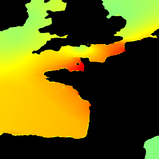
Maximum elevation of tide, note that Saint Malo and Bristol bay are indeed high tide places.
Note the green spot (hum, hard to see) corresponing to the amphidromic points north of France.
The animation of the full domain:

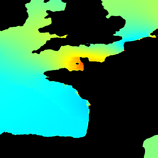
A zoom in "La Manche"

of the wave elevation. Dark blue is -2 metres and less. Dark red is +2 metres and more.](./maree_bretagne/eta-zoom.png)


A zoom on Daouhet and Erquy

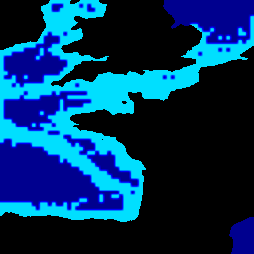
adaptation level

## Results tides
From "Table des Marées des Grands Ports du Monde", SHOM 1984, the sun and moon contribution are:
$$\frac{\text{Z0}}{100} + \frac{\text{AM2} \cos \left(\frac{1}{180} \pi \left(-\text{GM2}+2
\left(\text{h0}+\left(\frac{\text{heure}}{24}+13270\right) \text{hp0}\right)-2
\left(\left(\frac{\text{heure}}{24}+13270\right) \text{sp0}+\text{s0}\right)+30
\text{heure}\right)\right)+\text{AS2} \cos \left(\frac{1}{180} \pi (30
\text{heure}-\text{GS2})\right)}{1000}$$
with the parameters for Brest
$$
\{\text{Z0}\to 445,\text{AM2}\to 2160,\text{GM2}\to 142,\text{AS2}\to 755,\text{GS2}\to
182\}$$
and astronomical parameters
$$
\{\text{s0}\to 78.16,\text{sp0}\to 13.1764,\text{h0}\to 279.82,\text{hp0}\to 0.985647\}
$$
So that the value of the tide in Brest from the SHOM table the 1st of August 2017 (time in TU+1) is
$$Z(t)= Z_0 + AS_2 \cos(GS_2- WS_2 t) +
AM_2 \cos(GM_2 - WM_2 t)$$
with Moon parameters amplitude $AM_2=2.16$, phase $GM_2=5642.320805440571$, period
$WM_2=0.5058680493365497/60$ which is 12h25min14s (low tide to hight tide 6h12m37s) 44714.1643s (745.2360 min)
and sun parameters
$WS_2=0.5235987755982988/60$ which is 12 hours, (low tide to hight tide 6h)
$AS_2 =0.755$m the amplitude $GS_2 = 3.1764992386296798$ the phase shift
and mean height $Z_0=4.45$m
here we just plot the tide from SHOM, it shows the influence of sun
~~~gnuplot maree a Brest deux premiers modes le 1er Aout 2017 pendant un jour
set xlabel "t in min"
set ylabel "h in m"
Z0=4.45
AM2=2.16
AS2 =0.755
h1(x)=AS2*cos(3.1764992386296798 - 0.5235987755982988*x/60)
h2(x)=AM2*cos(5642.320805440571 - 0.5058680493365497*x/60)
p[0:24*60]Z0+h1(x)+h2(x) t'maree Brest SHOM 2 modes' w l, Z0+h2(x) t'onde M2 uniq.'
~~~
Plot of the tide in Brest and height at the boundary condition, the phase shift and amplitude of the left BC have been adjusted to fit more or less the tide in Brest
~~~gnuplot au large (condition d'entree)
set xlabel "t in min"
set ylabel "h in m"
p[0:]'large.txt' w lp,'brest.txt' w lp, h2(x) t'onde M2 uniq.'
~~~
Once, the phase shift and amplitude of the left BC have been adjusted in `radiation` BC, we check that the computed M2 tide in Saint Malo is not so far from the SHOM the 1st of August 2017
$$Z(t)= Z_0 +
AM_2 \cos(GS_2 - WM_2 t)$$
$Z_0=6.71$ m
with Moon parameters amplitude $AM_2=3.68$, phase is $GS_2=5643.47$, period
$WM_2=0.5058680493365497/60$
(we remove the $Z_0$ in the plot as we start by a mean constant level which takes into account the initial depth in the tiopography)
~~~gnuplot Brest calculé et Brest SHOM et Saint Malo Calculé et Saint Malo SHOM
set xlabel "t in min"
set ylabel "h in m"
sm2(x)= 3.68*cos(5643.47 - 0.505868*x/60)
p[0:][:7]'brest.txt' w lp, h2(x) t' Brest onde M2 uniq.','saintmalo.txt' w lp,sm2(x) t' SM onde M2 uniq.'
~~~
The Saint Malo is underpredicted, the tides are not synchronized with Brest as there is propagation in the channel.
Removing rotation decreases SM tide.
~~~gnuplot Brest calculé et Brest SHOM et Saint Malo Calculé et Saint Malo SHOM
set xlabel "t in min"
set ylabel "h in m"
sm2(x)= 3.68*cos(5643.47 - 0.505868*x/60)
p[64*60:24*3.5*60][:7]'brest.txt' w lp, h2(x) t' Brest onde M2','saintmalo.txt' w lp,sm2(x) t'SM onde M2'
~~~
Plot of tide in several harbours (with 'rotterdam.txt', which has to be checked); note amplification in Saint Malo, but little bit too small compared to reality.
Houat is in phase with Brest as expected (amplitude should be smaller).
~~~gnuplot
set key left
set xlabel "t in min (1day=1440min)"
set ylabel "h in m"
p[2000:5000][:8]'saintmalo.txt' w lp,sm2(x) t'SM M2','brest.txt' w lp,h2(x) t'B M2','houat.txt' w l,'manche.txt' w l,'rotterdam.txt'
~~~
# Links
* inspired/plagied from [tsunami 2004](http://basilisk.fr/src/examples/tsunami.c)
* see [http://basilisk.fr/src/examples/tides.c]()
* [http://gerris.dalembert.upmc.fr/gerris/examples/examples/tides.html]()
* [Gerris/modules/fes2004/]()
# bibliography
* [cours PYL](http://www.lmm.jussieu.fr/~lagree/COURS/MFEnv/)
* Phan et a. [Méthodologie pour la simulation de la marée avec la version 6.2 de TELEMAC- 2D et TELEMAC-3D](http://www.opentelemac.org/downloads/TRAINING%20AND%20TUTORIALS/simulation_maree_v6p2.pdf)
* SHOM Table des Marées des grands ports du Monde 1984
* "Tout savoir sur les marées" Odile Guérin/ Ouest-France/ 2004
* "La marée" B. Simon & A. Lahaye-Collomb, Les guides du SHOM 1997
* [La Marée (941-MOG), Les Guides du SHOM](http://www.shom.fr/les-produits/produits-nautiques/information-sur-les-ouvrages-nautiques/guides/)
* [Trois cents ans de mesures marégraphiques en France : (...) port de Brest, N. Pouvreau](https://tel.archives-ouvertes.fr/tel-00353660/document)
* PYL copie perso de "table des marées des grands ports du monde" du SHOM (1984) [tabledesmareesdesgrandsportsdumonde.pdf](https://mycore.core-cloud.net/index.php/s/5Y5mKjr1pWmj7aD)
* Jacques Bouteloup "[Vagues, marées, courants marins](https://books.google.fr/books?id=IXqJDwAAQBAJ)" Que sais-je, 1979
*/
/**
# notes
bug de formule en local sous macosx
~~~code
make maree_bretagne/plots;make maree_bretagne.c.html
sed -i -e 's/\\)//g' maree_bretagne.c.html;sed -i -e 's/\\(//g' maree_bretagne.c.html
sed -i -e 's/\\\[//g' maree_bretagne.c.html
sed -i -e 's/\\\]//g' maree_bretagne.c.html;
~~~
the simple
HTML tag works as well:
lien tout bête
un autre:
lien tout bête
*/