/**
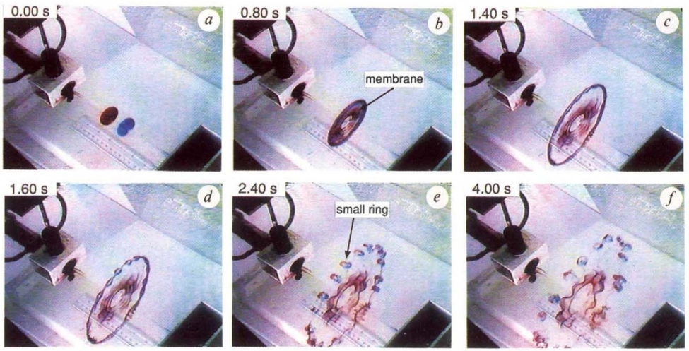
The experiment of [Lim and Nickels (1992)](https://www.nature.com/articles/357225a0).
# The collision of two vortex rings.
## Set-up
*/
#include "grid/octree.h"
#include "navier-stokes/centered.h"
#include "navier-stokes/perfs.h"
#include "fractions.h"
#include "view.h"
#include "lambda2.h"
#include "tracer-particles.h"
#include "scatter2.h"
#define RADIUS (sqrt(sq(y) + sq(z)))
Particles red, blue;
scalar f[];
int maxlevel = 11;
double ti = 4., ue = 0.008;
double Re = 1750.;
double tend = 120. + 0.1;
int np = 2e5;
/**
## Boundary conditions
Initially, there are two opposing jets at the `left` an `right`
wall. The `top` and `bottom` boundary can leak fluid.
*/
u.n[left] = dirichlet( f[] *(1.) * (t <= ti));
u.n[right] = dirichlet(-f[-1]*(1.) * (t <= ti));
u.n[top] = neumann (0.);
p[top] = dirichlet (0.);
pf[top] = dirichlet (0.);
u.n[bottom] = neumann (0.);
p[bottom] = dirichlet (0.);
pf[bottom] = dirichlet (0.);
int main() {
L0 = 32.;
X0 = Y0 = Z0 = -L0/2;
const face vector muc[] = {1./Re, 1./Re, 1./Re};
mu = muc;
run();
}
/**
The simulations starts when the jets are triggered. We have a guess at
an initial grid.
*/
event init (t = 0) {
refine (RADIUS < 2.5 && fabs(x) > 9.*L0/20. && level < (maxlevel - 1));
refine (RADIUS < 1.5 && fabs(x) > 19.5*L0/40. && level < (maxlevel));
f.refine = f.prolongation = fraction_refine;
fraction (f, 1. - RADIUS);
boundary ({f});
new_tracer_particles (0); //This should not be needed
}
/**
During the injection phase, the orifice shape is recomputed.
*/
event inject (i++; t <= ti) {
fraction (f, 1. - RADIUS);
boundary ({f});
}
/**
## Particles
Tracer particles are added as a sort of dye. This is done right after
the injection. Special care is taken to make this step MPI compatible.
*/
event add_tp (t = ti) {
if (pid() == 0) {
red = new_tracer_particles (np);
blue = new_tracer_particles (np);
int j = 0;
double Rseed = 1.8; //The rings are larger than the opening
while (j < np) {
double yp = noise();
double zp = noise();
if (sq(yp) + sq(zp) < sq(1.)) {
pl[red][j].x = X0 + fabs(noise()*ti*0.35);
pl[red][j].y = yp*Rseed;
pl[red][j].z = zp*Rseed;
pl[blue][j].x = X0 + L0 - fabs(noise()*ti*0.35);
pl[blue][j].y = yp*Rseed;
pl[blue][j].z = zp*Rseed;
j++;
}
}
} else {
red = new_tracer_particles (0);
blue = new_tracer_particles (0);
}
particle_boundary (red);
particle_boundary (blue);
set_particle_attributes (red);
set_particle_attributes (blue);
}
/**
## Output
Two movies are generated, plotting an adaptive $\lambda_2$-isosurface
value, a slice of the the cells and the the particles.
*/
event snapshots (t += 0.1) {
char str[99];
sprintf (str,"Re = %g", Re);
double val = -0.0001;
scalar l2[];
lambda2 (u, l2);
foreach()
l2[] = l2[] < val ? l2[] : nodata;
stats l2s = statsf(l2);
foreach()
l2[] = l2[] < val ? l2[] : 0;
boundary ({l2});
int w = 1280;
double tzoom = 100;
double fov = t < tzoom ? 15 - t/80 : 15 - t/80 - (t - tzoom)/2.5;
view (fov = 15 - t/80, width = w, height = 9*w/16, bg = {0.3, 0.4, 0.6},
theta = 0.6 + 0.15*cos(t/15), phi = 0.6, ty = 0.05);
isosurface ("l2", min (-l2s.stddev, val));
translate (y = -L0/4) {
cells (n = {0,1,0});
}
draw_string (str, pos = 2, lw = 3);
save ("movl2.mp4");
if (blue) {
clear();
view (bg = {0.9, 0.9, 0.9});
scatter (red, s = 7, pc = {0.8, 0.2, 0.2});
scatter (blue, s = 7, pc = {0.2, 0.2, 0.8});
translate (y = -L0/4) {
cells (n = {0,1,0});
}
draw_string (str, pos = 2, lw = 3);
save ("movp.mp4");
}
}
event dumps (t += 10) {
char fn[99];
sprintf (fn, "dump%g", t);
dump (fn);
sprintf (fn, "red_blue%g", t);
pdump (fn);
}
event adapt (i++)
adapt_wavelet ((scalar*){u}, (double[]){ue, ue, ue}, maxlevel);
event stop (t = tend);
/**
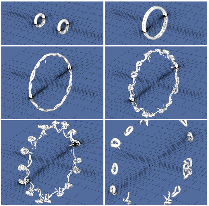
## Results
Visualization of the $\lambda_2$ iso-surface reveals detail:
See also via [vimeo](https://vimeo.com/284767041).
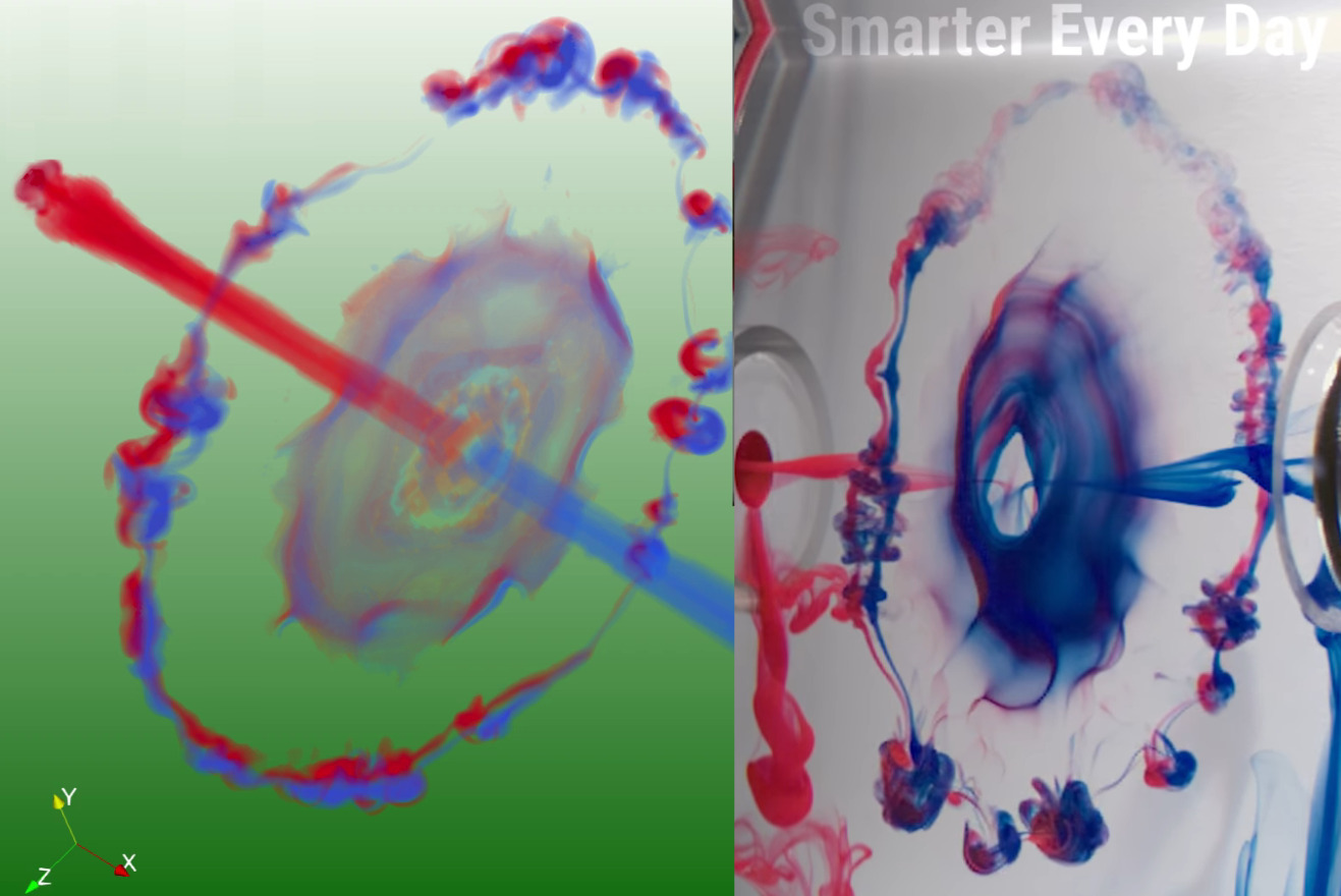
 There is also this visualization from another run with tracers:
 */
*/