sandbox/Antoonvh/rain.c
Sometimes it rains. Image courtesy of Quora.
Rain
The rain droplet concentration is an imporant metereological parameter. Therefore, we simulate the descent phase of some rain droplets on their journey towards the earth’s surface. The goal is to check wheater something interesting will happen. Furthermore, rain simulations are in high demand given that The Coding Train recieved about one million views on the linked video. So it seems wise to ride this wave, taken a more physics-based approach.
Set-up
We use an idealized free-fall case where droplets fall trough a periodic domain over and over again. The simulation is based on solving the equations of two-phase fluid motion, including surface tension associated with the water-air interface.
#include "navier-stokes/centered.h"
#include "two-phase.h"
#include "tension.h"
Due to the aforementioned periodicity, there does not exist an effective vertical coordinate dependent gravity potential. Hence, we should not use the reduced gravity approach.
#define REDUCED 0
#if REDUCED
#include "reduced.h"
#endif

int maxlevel = 9;
int np = 5;
double tend = 50;
double uya;
double lambda=0.25;
FILE * fpo ;

int main(){
  fpo= fopen("out.out","w");
#if REDUCED
  G.y = -1.;
#endif

  mu1=0.001;
  mu2=0.001;
  rho1=1.;
  rho2=0.1;
  f.sigma=0.0005;
  N=1<<(maxlevel-3);
  X0=Y0=-L0/2;
  foreach_dimension()
    periodic(left);
  run();
}
Droplet initializaiton
A total number of np=5 droplets are initialized. Note that no two runs will be the same, because the starting locations and droplet sizes are rondomized.
event init(t=0){
  TOLERANCE=10E-4;
  srand(time(NULL));
  double p[3]; // for xp,yp,R
  for (int j=1;j<=np;j++){
# if _MPI
    if (pid()==0){
# endif
      p[0]=0.47*noise();
      p[1]=0.47*noise();
      p[2]=0.01*fabs(noise())+0.02;
# if _MPI
    }
    MPI_Bcast(&p,3,MPI_DOUBLE,0,MPI_COMM_WORLD);
# endif
    double xp=p[0];
    double yp=p[1];
    double R=p[2];
    refine(level<maxlevel && sq(x-xp)+sq(y-yp)<sq(R+0.05));
    scalar f1[];
    fraction (f1,sq(R)-sq(x-xp)-sq(y-yp));
    foreach()
      f[]+=f1[];
  }
  foreach()
    f[]=min(f[],1.);
}
Drag
As the droplets descent, ‘air’ is being entrained in a downwards direction. In order to prevent a run-away of vertical velocities we add a drag force to the airy-phase.
#if !REDUCED
event acceleration (i++) {
  face vector av = a;
  uya=0;
  double surf=0;
  foreach(reduction(+:uya) reduction(+:surf)){
    uya+=u.y[]*(1.-f[])*sq(Delta);
    surf+=sq(Delta)*(1.-f[]);
  }
  uya=uya/surf;
  foreach_face(y)
    av.y[] -=(f[0,1]+f[])/2.+((2.-f[]-f[0,1])*(u.y[0,1]+u.y[])*fabs(uya)*lambda);
}
#endif
Adaptation
By adding two lines of code, the grid is adapted based on the estimated discretization error in the representation of the volume fraction field and velocity-component fields.
event adapt (i++)
  adapt_wavelet((scalar*){f,u},(double[]){0.001,0.05,0.05},maxlevel);
Output
Two animated gifs are generated.
event end(t=tend){}
event output(t+=0.1;t<=tend){
  char name1[100];
  sprintf(name1,"ppm2gif>f.gif");
  static FILE * fp = popen(name1,"w");
  sprintf(name1,"ppm2gif>lev.gif");
  static FILE * fpl = popen(name1,"w");
  scalar lev[];
  int n=0;
  foreach(reduction(+:n)){
    n++;
    lev[]=level;
  }
  output_ppm(f,fp,n=512, min = 0, max = 1,);
  output_ppm(lev,fpl,n=512, min = 2, max = maxlevel);
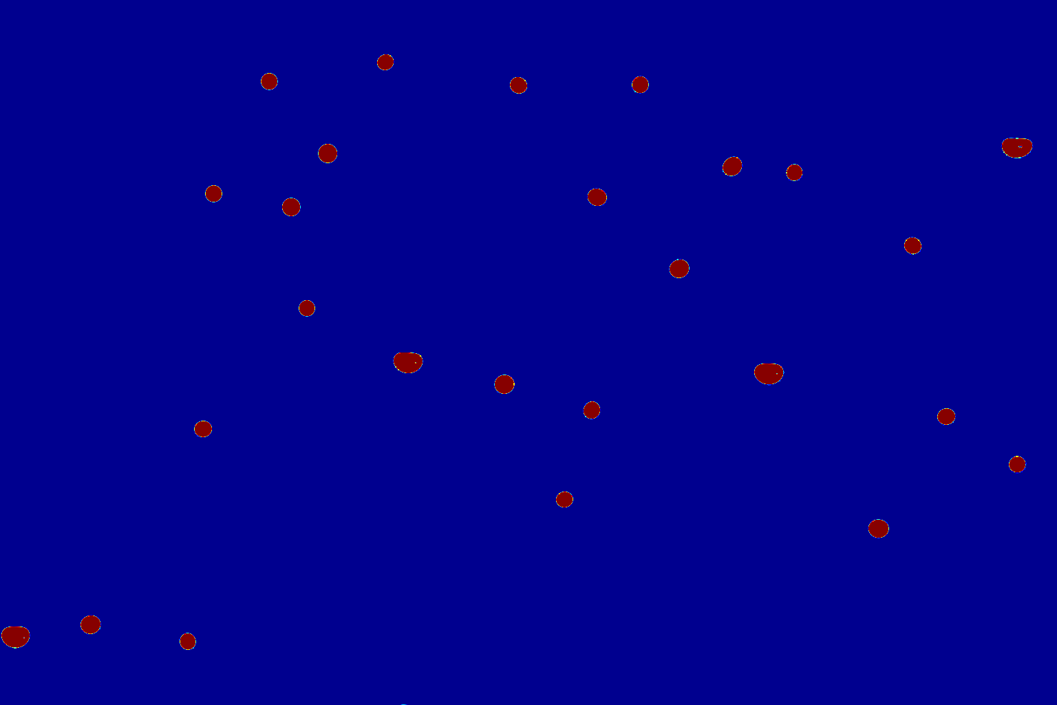
They reveal the dynamics of the droplets,

Rain
We observe that droplets can merge on their descent. This seems promoted by a two stage process. First droplets move into the wake of other droplets because of the lowered wake pressure. Second, because the drag force on the droplet is reduced a droplet may catch-up on its leading droplet and merge.
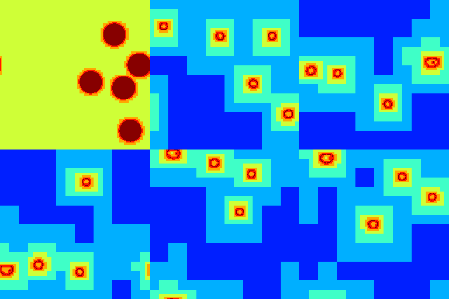
We also display the used adaptive grid,

grid
It appears that the algorithm focusses the computational resources on the droplets’ interfaces. We can check the compression ratio \Pi, that is defined as the ratio between the number of grid cells an equdistant static grid would have with the same maximum resolution and the used number of grid cells (i.e. \Pi > 1).
  if (pid()==0){
    printf("%d\t%g\t%d\t%g\t%g\n",i,t,n,uya,(double)((1<<(maxlevel*2))/n));
    fprintf(fpo,"%d\t%g\t%d\t%g\t%g\n",i,t,n,uya,(double)((1<<(maxlevel*2))/n));
  }
Here is the plot,
  set ylabel 'Pi'
  set xlabel 'time'
  set key off
  plot 'out.out' u 1:5 w l lw 3
The grid is coasened as the number of droplets decreases over time. (script)
That is truly the essence of having an adaptive grid, since there was no way of knowing on forehand where, when and how much the grid should be refined. Well done adapt_wavelet() function!
}
