lid.c

The Lid-Driven Cavity in 2D
- Results

The Lid-Driven Cavity in 2D

We study the flow in a lid-driven square cavity at different Reynolds numbers. The set-up consists of a square (L \times L) no-slip box with a top lid that forces a flow by moving in the positive x-direction with velocity U. Given a fluid viscosity (\nu), we can define a Reynolds number:

\displaystyle Re=\frac{UL}{\nu}.

Expressed in advection time scales we run the simulation until t_{end}=20 \times L/U.

in particular we are interested in how the computational costs scale with increasing Reynolds number. In the case set-up we use a normalized lengthscale L and lid velocity U.

#include "navier-stokes/centered.h"
scalar omg[],lev[],U[];
int maxlevel,m;
double vis,e,ens,vit,vir,vil,vib;

int main(){
  L0=1.;
  X0=Y0=0.;

We run the simulation 5 times (only 4 in the sandbox) with an increasing Reynolds number and maximum grid resolution.

  for (m=0;m<4;m++){
    run();
  }
}

The boundary conditions are chosen to be a no-slip box with a top lid that drives the flow.

u.t[top]=dirichlet(1.);
u.t[bottom]=dirichlet(0.);
u.n[left]=dirichlet(0.);
u.n[right]=dirichlet(0.);
u.t[left]=dirichlet(0.);
u.t[right]=dirichlet(0.);
u.n[top]=dirichlet(0.);
u.n[bottom]=dirichlet(0.);

event init(t=0){

The Reynolds number is directly controlled by the viscosity of the fluid \nu. The Reynolds number and maximum grid resolution are doubled each run iteration, starting with Re=125 and an effective resolution of 64\times64 grid points.

  vis=1./(125.*pow(2.,(double)m));
  maxlevel=6+m;

The grid is initialized consistent with the adaptation algorithm.

  init_grid(1<<3);
  const face vector muc[]={vis,vis};
  mu=muc;
  fprintf(ferr,"Re = %g and max res = %d X %d\n",1/vis,(int)pow(2,maxlevel),(int)pow(2,maxlevel));
  int j = 0;
  int g = 0;
  g=adapt_wavelet((scalar *){u},(double []){0.005,0.005},maxlevel,3).nf;
  boundary(all);
  while(g>1){
    foreach()
      u.x[]=0.;
    boundary(all);
    j++;
    fprintf(ferr,"j=%d and g=%d\n",j,g);
    g=adapt_wavelet((scalar *){u},(double []){0.005,0.005},maxlevel,3).nf;
  }
  DT=0.01;
}

For Re=500 we output an animation of the vorticity and the grid resolution.

event movie(t+=0.1){
  if (m==2){
    fprintf(ferr,"%g\n",t);
    foreach(){
      omg[]=((u.x[0,1]-u.x[0,-1]) - (u.y[1,0]-u.y[-1,0]))/(2*Delta);
      lev[]=level;
    }
    boundary({omg}); //For interpolation purposes
    static FILE * fp3 = popen ("ppm2gif > omg.gif", "w");
    output_ppm(omg,fp3, n=512,linear=true, min=-10., max=10.);
    static FILE * fp2 = popen ("ppm2gif > lev.gif", "w");
    output_ppm(lev,fp2, n=512, min=3, max=maxlevel);
  }
}

event adapt(i++){
  adapt_wavelet((scalar *){u},(double []){0.005,0.005},maxlevel,3);
}

At t=20L/U the simulation is stopped and some output statistics are calculated.

event stop(t+=1.;t<25.){
  if (t>=20.){
    ens=0;
    vit=0;
    vir=0;
    e=0;
    foreach(reduction(+:ens) reduction(+:e)){
      omg[]=((u.x[0,1]-u.x[0,-1]) - (u.y[1,0]-u.y[-1,0]))/(2*Delta);
      ens+=sq(omg[])*sq(Delta);
      lev[]=level;
      U[]=sqrt(sq(u.x[])+sq(u.y[]));
      e+=sq(U[])*sq(Delta);
    }
    boundary({omg});
    foreach_boundary(top)
      vit+=Delta*omg[];
    foreach_boundary(right)
      vir+=Delta*omg[];
    foreach_boundary(left)
      vil+=Delta*omg[];
    foreach_boundary(bottom)
      vib+=Delta*omg[];
    fprintf(ferr,"%d\t%g\t%g\t%g\t%g\t%g\t%g\t%g\n",i,t,e,ens,vit,vir,vir,vib);
    return 1;
  }
}

Results

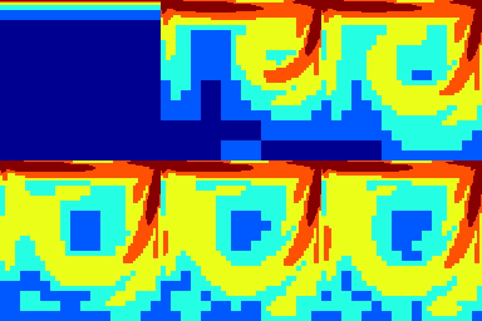
First we look at the evolution of the voricity field for Re=500 and the level of refinement within the domain.

Evolution of the vorticity field

Level of refinement

It appears that the costs of the simulations scale with Re^{1.9}. See the Appendix of Van Hooft et al. (2018) for a more elaborate narrative.